| #### SIDEBAR - Exploration of Control System Performance Criteria |
| ### 1. Stability |
| #### Definition and Importance Stability is the cornerstone of control system performance. A system is considered stable if, in response to a bounded input, it produces a bounded output. In practical terms, this means the system will not exhibit runaway behavior or oscillations that grow indefinitely over time. |
| #### Mathematical Representation - BIBO Stability: A system is Bounded-Input Bounded-Output (BIBO) stable if every bounded input produces a bounded output. Mathematically, if $ |x(t)| < M < $ for all $ t $, then $ |y(t)| < N < $ for all $ t $, where $ x(t) $ is the input, $ y(t) $ is the output, and $ M, N $ are constants. - Routh-Hurwitz Criterion: This criterion provides a method to determine the stability of a system by examining the location of the poles of the system’s transfer function. If all poles are in the left-half of the complex plane, the system is stable. |
| #### Practical Considerations - Stability Margins: In design, it’s not just about achieving stability, but ensuring a degree of robustness in stability, known as stability margins. These margins indicate how much a system’s parameters can vary before it becomes unstable. |
| ### 2. Transient Response |
| #### Characterizing Transient Behavior Transient response refers to the system’s reaction from an initial state to reaching its steady state. Key characteristics include: - Rise Time: Time taken for the response to rise from 10% to 90% of its final value. - Settling Time: Time taken for the response to stay within a certain percentage (commonly 2% or 5%) of the final value. - Overshoot: The amount by which the response exceeds the final value. - Damping Ratio: A measure of the oscillations in the response. |
| #### Design Objectives - Speed of Response: A faster rise time is often desirable, but can lead to increased overshoot. - Oscillation Control: Minimizing overshoot and ensuring the system settles quickly without prolonged oscillations. |
| ### 3. Steady-State Accuracy |
| #### Understanding Steady-State Once transient effects have diminished, a system enters steady-state. Here, the output should ideally match the commanded value as closely as possible. |
| #### Measures of Steady-State Accuracy - Error Metrics: Common measures include steady-state error, tracking error, and error constants like position, velocity, and acceleration error constants. - System Type and Error: The type of control system (Type 0, Type 1, etc.) determines its ability to handle different kinds of steady-state errors, particularly for step, ramp, and parabolic inputs. |
| #### Designing for Accuracy - Feedback Control: Incorporating feedback effectively reduces steady-state error. - Integral Control: Adding an integral component can eliminate steady-state error for certain types of inputs. |
| ### 4. Sensitivity and Robustness |
| #### Resilience to Variations Sensitivity and robustness measure a system’s ability to maintain performance despite changes in system parameters or environmental conditions. |
| #### Quantitative Analysis - Sensitivity Function: This function quantifies how sensitive the system’s output is to changes in a particular parameter. - Robust Design Techniques: Methods like H-infinity and μ-synthesis are used to design systems that maintain performance over a range of uncertainties. |
| #### Practical Application - Worst-Case Analysis: Assessing system performance under extreme variations to ensure robust operation. |
| ### 5. Disturbance Rejection |
| #### Minimizing External Impact Control systems often operate in environments with external disturbances. Effective disturbance rejection minimizes the impact of these disturbances on the system’s output. |
| #### Evaluating Disturbance Rejection - Transient Response to Disturbance: Observing how quickly and effectively the system mitigates the impact of a disturbance. - Steady-State Error due to Disturbance: Ensuring that, in steady-state, the disturbance has minimal or no impact on the output. |
| #### Control Strategies - Feedforward Control: Anticipating disturbances and compensating for them before they affect the system. - Feedback Control: Adjusting system behavior in response to disturbances detected in the output. |
| — END OF SIDEBAR |
| ## Transition to Quantitative Specifications |
| In control system design, we often start by specifying: - the desired transient - and steady-state accuracy. |
| Once a system is designed with these specifications, we then evaluate its performance in terms of robustness and disturbance rejection. |
| Note: Current research in control system design is evolving towards including sensitivity and robustness in the initial design phase itself. However, this is still an emerging area and not widely incorporated in standard curricula. We will focus on the classical way of control design, and this will provide the base to understand robustness and sensitivity. |
| ### Classical Approach in Control System Design |
| In the traditional methodology of control system engineering, the primary focus is initially set on transient and steady-state accuracy. This methodical approach encompasses several key steps: |
| 1. Assurance of System Stability: This initial phase involves the application of analytical tools such as the Routh stability criterion. These tools are employed to ascertain the stability conditions of the system by determining the specific ranges of parameters that ensure stability. The stability of the system is a primary requirement. If this does not hold everything else does not matter. |
| 2. Optimization for Transient and Steady-State Performance: The next step is the careful selection of system parameters. These parameters are chosen from within the identified stability domains with the objective of achieving the desired levels of transient and steady-state accuracy. This selection process is crucial for the system to respond effectively to changes and maintain accuracy over time. This is the quantitative specification of the system performance. |
| 3. Assessment of Robustness and Disturbance Rejection Capabilities: The final phase involves a thorough simulation of the control system. This simulation is critical to evaluate whether the system meets predefined standards for robustness and its ability to reject disturbances. If these standards are not met, it triggers a re-evaluation and redesign of the control strategy. This iterative nature of design acknowledges that achieving optimal performance often requires multiple adjustments and refinements. |
| By following these steps, the classical approach ensures a comprehensive and iterative development process, aiming to create a control system that is stable, accurate, robust, and capable of effectively rejecting disturbances. |
| ### Design Methodology for Control System: Stability, Accuracy, and Robustness Assessment |
| 1. Identifying Stability Domains of Parameters: - The initial step in the design of a control system involves determining the conditions under which the system will remain stable. - Stability, in control systems, means that the system will not exhibit unbounded or erratic behavior in response to a given input. - To find these conditions, we use analytical methods like the Routh stability criterion. This criterion helps in identifying the ‘domains’ or ranges of system parameters (like gain, damping ratio, etc.) that ensure the system remains stable. - For example, we might solve problems where we manipulate one or two parameters (like adjusting the gain of a controller) to see how these changes affect system stability. |
| 2. Ensuring Transient and Steady-State Accuracy: - Once we’ve identified the stability domains, the next step is to refine the system parameters within these domains. - This refinement aims to achieve specific performance goals related to how the system responds over time (transient performance) and how accurately it maintains its output in the long term (steady-state performance). - Transient accuracy involves how quickly and effectively the system responds to changes, while steady-state accuracy focuses on how closely the system’s output matches the desired output after initial fluctuations have settled. |
| 3. Evaluating Robustness and Disturbance Rejection: - After satisfying the transient and steady-state requirements, we return to the original system configuration. - Here, we simulate the system under various conditions to assess its robustness (how well it performs under different operating conditions or parameter variations) and its ability to reject disturbances (how well it maintains its performance in the presence of unexpected external influences). - If the system fails to meet the robustness or disturbance rejection criteria, the design process may need to be revisited. This might involve adjusting the parameters again or even redesigning certain aspects of the system. |
| By following this structured approach, we ensure that the control system we design is not only stable but also meets specific performance criteria in both the short and long term, and is resilient to external disturbances and internal parameter changes. This comprehensive evaluation is crucial for creating a reliable and efficient control system. |
| ## Exploring Transient Performance Specifications |
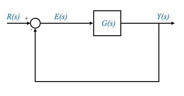
| ### Unity-Feedback Systems |
| For simplicity, we’ll consider a unity-feedback system, though the principles apply to non-unity-feedback systems as well. |
|
| - The system transfer function is: |
| \[ Y(s) / R(s) = G(s) / (1 + G(s)) \] |
| - Here, $ Y(s) $ is the output, $ R(s) $ is the input, and $ G(s) $ is the system’s transfer function. |
| ### Nature of Input Signals |
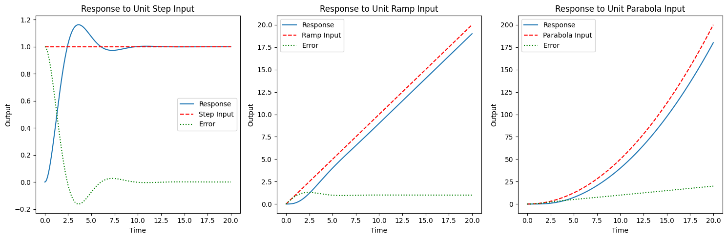
| In practical control systems, the nature of the input signal is unpredictable. Therefore, we use standard test signals (step, ramp, parabola) to design and evaluate the system. If they system performs well for these signals, it should perform well for any other signal. |
| The transient performance is depended by the system’s poles and is relatively independent of the input signal’s nature. |
| For example, if the poles are on the LHP, the transient will die out. The transient hence is dependent on the system’s characteristic and not on the specific input. |
| In other words, in control system design, it’s crucial to evaluate how the system will respond to various types of input signals. Since it’s impractical to predict every possible input a system might encounter in real-world operations, we use standard test inputs as benchmarks. These include step, ramp, and parabolic signals, among others. |
| - Step Input: This is a sudden change, typically from zero to a fixed value. It’s useful for observing the system’s immediate reaction and its transient response characteristics. |
| - Ramp Input: This input increases linearly over time, representing a continuously changing setpoint. It helps in understanding how the system tracks a gradually varying input and can be particularly revealing for systems where the rate of change of the input is significant. |
| - Parabolic Input: This represents a scenario where the input changes at an accelerating rate, providing insights into how the system handles more complex, dynamically changing conditions. |
| The choice of these test signals is not arbitrary. They are selected because they effectively excite different aspects of the system’s behavior. The step input tests the system’s basic stability and transient response. The ramp input examines the system’s ability to keep up with a continuously changing setpoint, which is crucial for tracking performance. The parabolic input, by introducing an accelerating change, challenges the system’s responsiveness to more complex and dynamic inputs. |
| By designing a control system that performs satisfactorily with these standard test inputs, we can infer that it will likely handle a wide range of real-world inputs effectively. This approach simplifies the design process by reducing the infinite variety of possible inputs into a manageable set of standard tests, each focusing on a critical aspect of system performance. |
| ### Utilizing Step Input for Transient Response Analysis |
| - In the context of transient response analysis, the step input, represented by a unit-step function $ (t) $, is commonly employed. - The underlying reasoning for this choice is that a step input is particularly effective in stimulating all the modes of the system. This comprehensive excitation enables a detailed observation and analysis of the system’s transient response. It’s important to note that the stability and transient characteristics of a control system are primarily determined by the locations of its poles, which are inherent properties of the system itself, rather than the nature of the input signal. Therefore, by using the simplest form of test input, the step input, we can efficiently evaluate the system’s behavior without the need for more complex input forms. This approach simplifies the analysis while still providing a thorough understanding of the system’s transient dynamics. |
| For this reason, the unit-step input is used to quantitatively specify the transient characteristics of the system. Note also that a larger ampliture does not change the nature of the response, it will only change the amplitude of the response. |
|
| 🤔Pop-up Question: Why do we prefer a unit-step input for transient analysis? |
| Answer: A unit-step input simplifies the analysis and is effective in exciting all system modes, making it ideal for observing the transient behavior of the system. |
| ## Steady-State Performance Specifications |
| ### Dependency on Input and System Characteristics |
| Unlike transient performance, the steady-state response depends on both the system characteristics and the nature of the input signal. Therefore, a single type of input signal may not suffice to fully characterize steady-state performance. |
| Ideally, to thoroughly characterize the steady-state behavior, the actual input that the system will encounter in real-world operations would be required. However, in practical scenarios, this specific input may not always be predetermined or known in advance. As a result, the necessity arises to utilize standardized test signals. These test signals serve as proxies to approximate a range of possible real-world inputs, thereby enabling a more robust evaluation of the system’s steady-state performance under various hypothetical conditions. |
| ## Dealing with Unknown Inputs in Control Systems |
| ### Real-World Examples and the Challenge of Unpredictable Inputs |
| When designing control systems, we often face the challenge of unknown or variable inputs. Let’s explore this through a few examples: |
| #### Example 1: Tracking Radar System - Scenario: A radar system designed to track aircraft movements. - Challenge: Predicting the exact motion profile of the aircraft is nearly impossible. The system must be adaptable to various possible trajectories. |
| #### Example 2: Numerical Control of Machine Tools - Situation: Machines designed for cutting or shaping materials. - Complexity: The machine could be required to perform a range of tasks, from tapering to cutting parabolic profiles. The system must handle any shape it’s tasked with. |
| #### Example 3: Residential Heating System - Condition: Variability in environmental temperatures across seasons. - Impact: This variation significantly changes the disturbance signals the system must handle, from summer to winter. |
| In each of these cases, the control system’s input and the disturbance signals it encounters cannot be precisely predetermined. This uncertainty directly affects the steady-state performance, which is inherently dependent on the nature of the input. |
| ### Addressing Unpredictable Inputs |
| #### Polynomial Representation of Inputs |
| To overcome the challenge of unpredictable inputs, a strategy is to represent the actual input as a sum of polynomial functions. Mathematically, any complex function can be decomposed into a series of simpler polynomial functions. Thus, ensuring satisfactory performance for a range of polynomial inputs can provide confidence that the system will perform well for various real-world inputs. |
| - Polynomial Function Representation: |
| According to the previous discussion we can see the input \(r(t)\) as a generic polynomial function indexed by \(k\): |
| \[ r(t) = \frac{1}{k!} t^k \mu(t) \] |
| Here, $ r(t) $ is a polynomial function of time, $ k $ is the order of the polynomial, and $ (t) $ is the unit-step function. |
| #### Standard Polynomial Inputs for Steady-State Performance |
| For different values of $ k $, we get various standard test inputs: |
| - $ k = 0 $: $ r(t) = (t)$ becomes a unit-step function. - $ k = 1 $: $ r(t) = t (t)$ represents a ramp function. - $ k = 2 $: $ r(t) = t^2(t)$ forms a parabolic function. |
| As $ k $ increases, the input becomes faster, but in practical scenarios, values of $ k $ beyond 2 are rarely needed. This is because real-world system inputs are generally not as fast as higher-order polynomials. Therefore, in most cases, satisfying the performance criteria for $ k = 1 $ (ramp function) and $ k = 2 $ (parabolic function) is sufficient. |
| #### Practical Considerations in Control Design |
| - Complexity and Stability: As the order $ k $ increases, control system design becomes more challenging, particularly regarding maintaining stability. For $ k > 3 $ maintaining stability is very difficult. |
| - Industrial Relevance: For many industrial applications, a value of $ k = 1 $ is often sufficient, aligning with practical requirements. |
| Moving forward, our analysis will concentrate on three fundamental test inputs, each characterized by their unique time-dependent behavior and their distinctive “unit” nature, derived from the property that their derivatives are scaled to unity: |
| 1. Unit-Step Function: - Mathematical Representation: $ r(t) = (t) $ - Characteristics: This function represents a sudden change at $ t = 0 $, transitioning sharply from 0 to 1. It is termed ‘unit-step’ because its derivative, a delta function, peaks at unit height. |
| 2. Unit-Ramp Function: - Expression: $ r(t) = t (t) $ - Description: This linearly increasing function symbolizes a ramp input that starts at $ t = 0 $ and increases at a constant rate. The ‘unit’ designation is due to its derivative being constant (unity) over time. |
| 3. Unit-Parabola Function: - Formulation: $ r(t) = t^2 (t) $ - Explanation: This function represents a parabolic curve, starting at $ t = 0 $ and increasing quadratically over time. The factor \(\frac{1}{2}\) ensures that the derivative of this function, $ t (t) $, aligns with the unit-ramp function, hence the term ‘unit-parabola’. |
| Each of these inputs serves as a standard test signal in control systems analysis, providing a basis for examining system responses under different types of input scenarios. |
| ## Transient Performance Specifications |
| ### Industry-Based Approach |
| Instead of relying solely on mathematical models, an industry-based approach involves examining real-world control systems. By exciting these systems with a standard step input and observing their response, we can derive practical transient performance specifications. |
| ### Observations and Indices for Transient Performance |
| - Typical Response: The transient response of a practical control system often exhibits damped oscillations before reaching steady state. |
|
| - Acceptability of Oscillations: Some overshoot is generally acceptable in practical scenarios. |
| ### Key Performance Indices |
| 1. Rise Time ($ t_r $): This is the duration required for the system’s response to initially reach the final value (or steady-state level) 100% for the first time. It provides insight into the response speed of the system following a change. |
| 2. Peak Overshoot ($ M_p $): This parameter measures the maximum level by which the system’s response exceeds its final value. If the peak overshoot is within acceptable limits, it is generally assumed that any subsequent fluctuations in magnitude will also be acceptable, as they are typically smaller. |
| 3. Peak Time ($ t_p $): This refers to the time elapsed from the initiation of the response until it reaches its maximum overshoot. It indicates how quickly the system reaches its peak response following a disturbance or a change. |
| 4. Settling Time: This is the time required for the system’s response to consistently remain within a specific tolerance range around the final value. The tolerance range, often set at 2% or 5% of the final value, varies based on the accuracy requirements of the application. This metric is crucial for determining how quickly the system stabilizes following transient fluctuations. |
| #### Additional Note on Mathematical Characterization of Settling Time: |
| Consider a function of the form \(e^{-t/\tau}\), which represents an exponential decay. |
| Mathematically, such a function only completely settles as \(t\) approaches infinity (\(t \rightarrow \infty\)). |
| In other words, its theoretical settling time is infinite. However, in practical control system analysis and design, we define a settling time within a band of practical acceptability to reflect realistic operating conditions. This approach acknowledges that, in practice, a system is considered ‘settled’ when its response is close enough to the steady-state value, even if it hasn’t reached it exactly. |
| Finally, it is worth noticing that we will tackle steady-steady accuracy separately because it is not only specified for a unit-step but also for ramp and parabolic inputs. |
| Given these four parameters, we can almost reconstruct the step reponse. |
| ### Exploring Transient Dynamics in Second-Order Systems: An Interactive Simulation |
| We can see the effect of changing these parameters using the following python code. |
| #### Instructions for Use: |
| 1. Zeta Slider: Adjust this slider to change the damping ratio of the system. A lower value means less damping (more oscillatory response), and a higher value means more damping (less oscillatory response). 2. Omega_n Slider: This slider changes the natural frequency of the system. A higher natural frequency generally leads to a faster response. |
| 3. Sim Time Slider: This slider changes the simulation time. |
| With these sliders, you can observe how varying the damping ratio and natural frequency affects the transient response of a stable second-order system. |
| ::: {#8ee42504 .cell} ``` {.python .cell-code} # Import necessary libraries import numpy as np import matplotlib.pyplot as plt import control |
| def find_max_consecutive_index(arr): max_consecutive_index = None consecutive_start = None |
| for i in range(len(arr) - 1): if arr[i] + 1 != arr[i + 1]: if consecutive_start is not None: max_consecutive_index = consecutive_start consecutive_start = None elif consecutive_start is None: consecutive_start = i + 1 |
| # Check if the entire array is consecutive if consecutive_start is not None: max_consecutive_index = consecutive_start |
| return max_consecutive_index if max_consecutive_index is not None else len(arr) - 1 |
| # Define a function to calculate and plot the system response with performance parameters def plot_response(zeta, omega_n, sim_time): # System parameters: zeta (damping ratio), omega_n (natural frequency) num = [omega_n**2] # Numerator (assuming unit gain) den = [1, 2 * zeta * omega_n, omega_n**2] # Denominator |
| # Create a transfer function model system = control.tf(num, den) |
| # Time parameters t = np.linspace(0, sim_time, int(sim_time*100)) # Time vector |
| # Step response t, y = control.step_response(system, t) steady_state_value = y[-1] |
| # Rise Time rise_time_indices = np.where(y >= steady_state_value)[0] rise_time = t[rise_time_indices[0]] if rise_time_indices.size else None |
| # Peak Overshoot and Peak Time peak_overshoot = np.max(y) - steady_state_value peak_time = t[np.argmax(y)] |
| # Settling Time (within 2% of steady-state value). This is found numerically. settling_time_indices = np.where(abs(y - steady_state_value) <= 0.02 * steady_state_value)[0] ts_index = find_max_consecutive_index(settling_time_indices) settling_time = t[settling_time_indices[ts_index]] if settling_time_indices.size else None |
| # Plot plt.figure(figsize=(10, 6)) plt.plot(t, y, label=‘System Response’) plt.axhline(steady_state_value, color=‘r’, linestyle=‘–’, label=‘Steady State’) # tolerange band (0.02 percent) plt.axhline(steady_state_value * 1.02, color=‘g’, linestyle=‘:’, label=‘Settling Time Bound’) plt.axhline(steady_state_value * 0.98, color=‘g’, linestyle=‘:’) |
| if rise_time: plt.axvline(rise_time, color=‘y’, linestyle=‘-’, label=f’Rise Time: {rise_time:.2f}s’) plt.axvline(peak_time, color=‘b’, linestyle=‘-’, label=f’Peak Time: {peak_time:.2f}s’) plt.scatter(peak_time, np.max(y), color=‘black’, label=f’Peak Overshoot: {peak_overshoot:.2f}’) |
| if settling_time: plt.scatter(settling_time, y[settling_time_indices[ts_index]], color=‘purple’) plt.axvline(settling_time, color=‘purple’, linestyle=‘-’, label=f’Settling Time: {settling_time:.2f}s’) |
| plt.title(‘Transient Response with Performance Parameters’) plt.xlabel(‘Time (seconds)’) plt.ylabel(‘Output’) plt.legend() plt.grid(True) plt.show() |
| # Interactive sliders from ipywidgets import interact, FloatSlider interact(plot_response, zeta=FloatSlider(value=0.3, min=0.01, max=1.0, step=0.01), omega_n=FloatSlider(value=2, min=1, max=10, step=0.1), sim_time=FloatSlider(value=10, min=1, max=50, step=1)) ``` |
| ::: {.cell-output .cell-output-display} |
{=html} <script type="application/vnd.jupyter.widget-view+json"> {"model_id":"95764ec2f5204f0a954d0b87d489585a","version_major":2,"version_minor":0,"quarto_mimetype":"application/vnd.jupyter.widget-view+json"} </script> |
| ::: |
| ::: {.cell-output .cell-output-display} |