Welcome to the next phase of our course on Principles of Automatic Control. In this notebook, we will delve into the Root Locus Design.
Let’s begin by revisiting some of the concepts we have previously discussed and then move on to practical design examples.
What is a Compensator?
A compensator is a type of controller, like PI (Proportional-Integral), PD (Proportional-Derivative), or PID (Proportional-Integral-Derivative), designed to enhance a system’s performance.
Performance in control systems is generally categorized into two types:
Transient Performance: How the system responds to changes over time, especially when it’s adjusting to reach its steady state.
Steady-State Performance: The system’s behavior once it has settled into a consistent pattern over time.
Transient performance is crucial because it determines how quickly and accurately the system reaches its desired state after a disturbance. Steady-state performance, on the other hand, is important for the long-term stability and accuracy of the system.
System Structure with Compensators
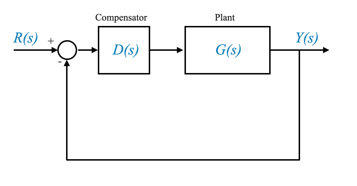
Let’s consider a typical control system structure:
The Plant: The core part of the system being controlled.
The Controller/Compensator: A device or algorithm that adjusts the plant’s output based on feedback.
In this setup, the compensator (\(D(s)\)) is placed in cascade with the plant. This arrangement can also be modified with minor feedback loops, which can be represented in a similar structural format for design purposes.
It’s vital to understand that the choice of compensator affects both the transient and steady-state behaviors of the system. A well-chosen compensator can significantly enhance the system’s response to changes and maintain stability over time.
Types of Compensators
Phase Lead Compensator
Definition and Transfer Function
A phase lead compensator is used to improve transient performance by shifting the root locus to the left, which enhances system stability. The transfer function of a phase lead compensator is given by:
\[ D(s) = K_c \frac{(s + z_c)}{(s + p_c)} \]
Where: - $ K_c $ is the gain. - $ z_c $ is the zero of the compensator. - $ p_c $ is the pole of the compensator.
Physical Realization: Often realized using an Op-Amp circuit with specific resistor and capacitor values determining $ z_c $, $ p_c $, and $ K_c $.
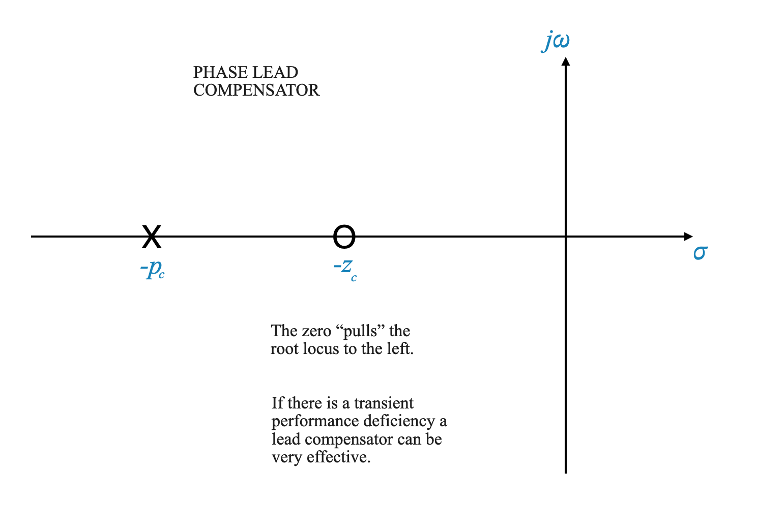
Figure: plot illustrating the pole-zero diagram of a phase lead compensator. The zero is at $ -z_c $ and the pole at $ -p_c $, with the pole farther from the origin than the zero.
Compensator Design Principles
The zero in the phase lead compensator (at $ s = -z_c $) introduces a derivative action, pulling the root locus plot towards the left half of the plane, thus enhancing stability and transient performance.
An additional pole is included for noise attenuation purposes, especially for high-frequency noise, represented by the pole at $ s = -p_c $.
Placement of the lead compensator is critical in cases where transient performance needs improvement.
The PD controller is a special case of a phase lead compensator that does not include the pole.
Pop-up Question: Why is a phase lead compensator used to improve transient performance? Answer: Because it shifts the root locus to the left, enhancing the system’s stability and transient response.
Example: Phase Lead Compensator
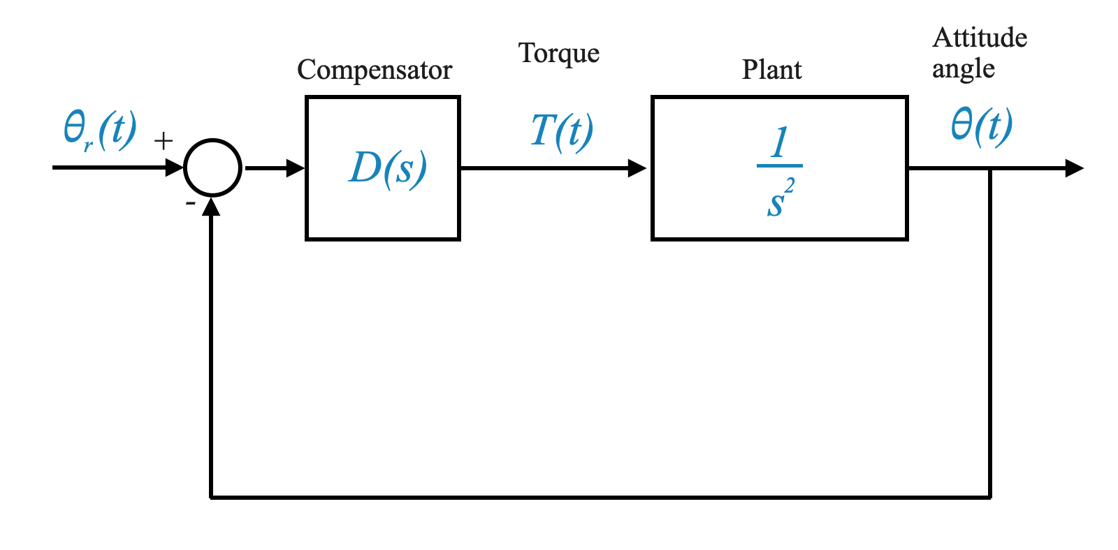
Let’s apply these concepts to a practical example: the attitude control of a satellite. The system can be modeled as $ $.
Scenario: Satellite Attitude Control
System Model:
\[ G(s) = \frac{1}{s^2} \]
Input: Torque $ T(t) $ Output: Attitude angle $ (t) $ System Type: Type-2 (implies good steady-state performance: zero error for step and ramp inputs, and finite error to acceleration inputs)
Problem Statement: Addressing instability due to a double integrator at the origin.
Initial System Design
We start considering the simple situation where
\[
D(s) = K
\]
This corresponds to the situation where \(D(s)=K\) is the constant of an actuator tht converts the elctrical signals into a torque \(T(t)\) for the thrusters.
Open-Loop Transfer Function:
\[ G(s) = \frac{K}{s^2} \]
Closed-Loop Behavior:
We can analyse it using the root locus as \(K\) varies.
Understanding the Root Locus Plot
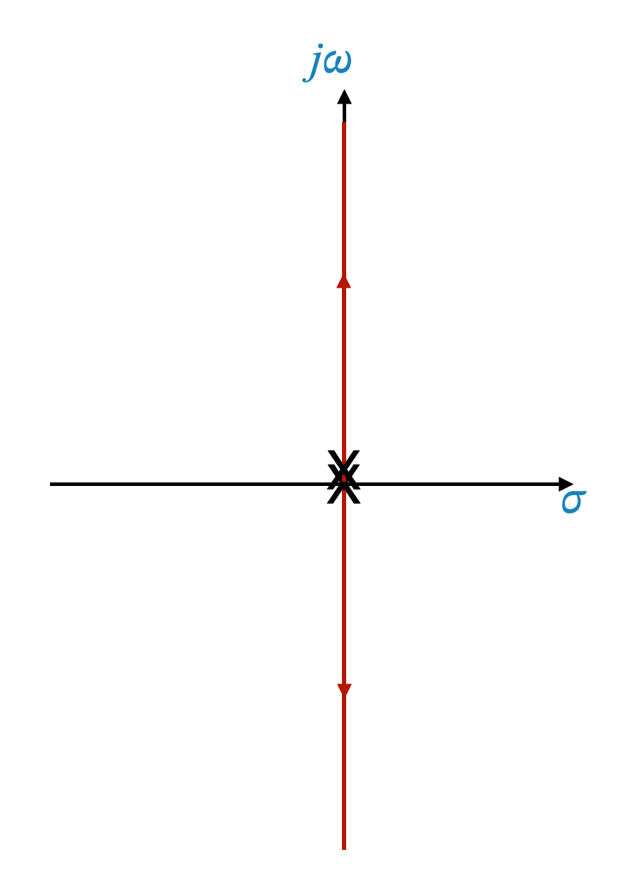
Remember, the root locus plot is a graphical representation of how the closed-loop poles of a control system vary with changes in a system parameter, typically the gain.
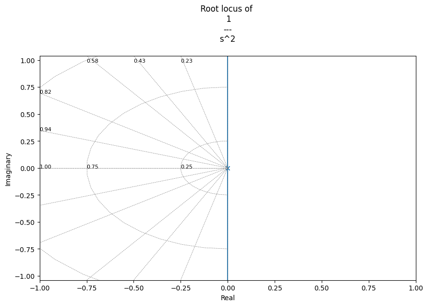
For the system $ $, the root locus plot indicates an oscillatory nature. This is because for all values of ‘s’, the roots lie on the imaginary axis of the s-plane, which is characteristic of undamped oscillations.
We can plot the root locus using Python in this way:
import numpy as npimport matplotlib.pyplot as pltimport control as ctlnumerator = [1]denominator = [1, 0, 0]G = ctl.TransferFunction(numerator, denominator)# Plot the root locusplt.figure(figsize=(10, 6))ctl.root_locus(G, plot=True);plt.title(f'Root locus of {G}');
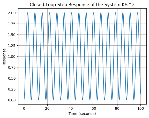
Here is a Python script that simulates the closed-loop system:
import numpy as npimport matplotlib.pyplot as pltimport control as ctl# System parametersK =1# You can modify this gain value as needed# Transfer function of the systemnumerator = [K]denominator = [1, 0, 0] # s^2 term has a coefficient of 1, s term is 0, constant term is 0system = ctl.tf(numerator, denominator)# Closed loop transfer function with a unity feedback# For a unity feedback system, the feedback transfer function is simply 1closed_loop_system = ctl.feedback(system, 1)# Time parameters for simulationt = np.linspace(0, 100, 1000) # Simulation from 0 to 10 seconds, with 1000 points# Step responset, y = ctl.step_response(closed_loop_system, t)# Plottingplt.plot(t, y)plt.title('Closed-Loop Step Response of the System K/s^2')plt.xlabel('Time (seconds)')plt.ylabel('Response')plt.grid(True)plt.show()
Decision Making in Compensator Design
Choosing Between Phase Lead and Phase Lag Compensator
Phase Lead Compensator: Ideal for improving transient performance by shifting the root locus to the left, enhancing stability.
Phase Lag Compensator: Adds another integrator to the system (or something very close to that), making it a type-3 system, which leads to instability. It’s typically used for improving steady-state accuracy. Modify the Python code above or plot the Root Locus for a type-3 system.
In our current scenario, the primary concern is not steady-state accuracy but transient performance. Therefore, a phase lead compensator is the preferred choice.
Implementing the Phase Lead Compensator
The Concept
The phase lead compensator is represented by the transfer function:
\[ D(s) = K_c \frac{(s + z_c)}{(s + p_c)} \]
where $ K_c $, $ z_c $, and $ p_c $ are the parameters we can determine to achieve our requirements.
Note: The concepts behind the design are more important than the specific design. More than one design can be suitable.
The Design Approach
System Representation: The plant’s transfer function is given by $ G(s) = $, where $ K $ is an adjustable gain. We can then take the compensator as $ $.
Implementation Considerations: Depending on the hardware, the gain $ K $ might be adjusted within the plant or through an external amplification stage in the compensator.
There are three parameters under our control. How we implement these parameters depend on the hardware.
We call $ $ as uncompensated system that in this case includes the design parameter \(K\).
Consider an attitude control system for a satellite: - Uncompensated System: \[ \frac{K}{s^2} \] - Compensator: \[ D(s) = \frac{s + z_c}{s + p_c} \]
Designing for Specific Performance Requirements
Translating Performance into Closed-Loop Pole Locations
Suppose the design requirements are a damping ratio $ = 0.707 $ and a settling time $ t_s = 2$ seconds. Our goal is to translate these requirements into desired closed-loop pole locations.
Remember that transient requirements might be given to you in terms of $_n $ (natural frequency), \(M_p\) (Overshoot Peak), etc.
Remember also that we can often go from one specific requirement to another. For example, we can calculate:
\[
\zeta\omega_n = \frac{4}{t_s} = 2
\]
The closed-loop pole locations can be determined from these values. Below the steps to do it.
To calculate the position of the desired closed-loop poles for a control system with a specified damping ratio $ $ and settling time $ t_s $, we use the standard formulas related to the second-order system’s response characteristics.
The desired closed-loop poles are generally complex conjugates for underdamped systems, and their position in the s-plane is determined by the damping ratio $ $ and the natural frequency $ _n $.
Given: - Damping ratio $ = 0.707 $ - Settling time $ t_s = 2 $ seconds
**Calculate the Natural Frequency ($ _n $)**: The settling time for a second-order system is approximated by $ t_s $. We rearrange this to solve for $ _n $:
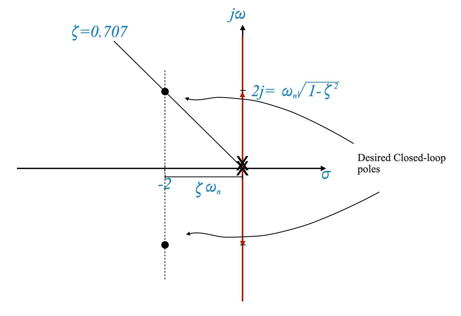
Determine the Real and Imaginary Parts of the Poles: The general form of the closed-loop poles for a second-order system is:
\[ s = -\zeta \omega_n \pm j\omega_n\sqrt{1 - \zeta^2} \]
The real part (sigma) is given by $ -_n $ and the imaginary part (omega) by $ _n $.
Calculating these:
Real Part: $ -_n = -0.7 $
Imaginary Part: $ _n = 2.857 $
Closed-loop Pole Locations: Therefore, the closed-loop poles are located at approximately:
\[ s = -2 \pm j2 \]
These calculations give you the desired locations for the closed-loop poles in the s-plane to achieve the specified damping ratio and settling time in your control system design.
We can plot this on the s-plane:
Figure: Plot of the root locus of the uncompensated system. It is possible to identify where the closed-loop poles should be for the desired performance.
We need to modify the behaviour of the root locus to pass through the desired closed-loop poles so that the requirements on the transient accuracy are satisfied.
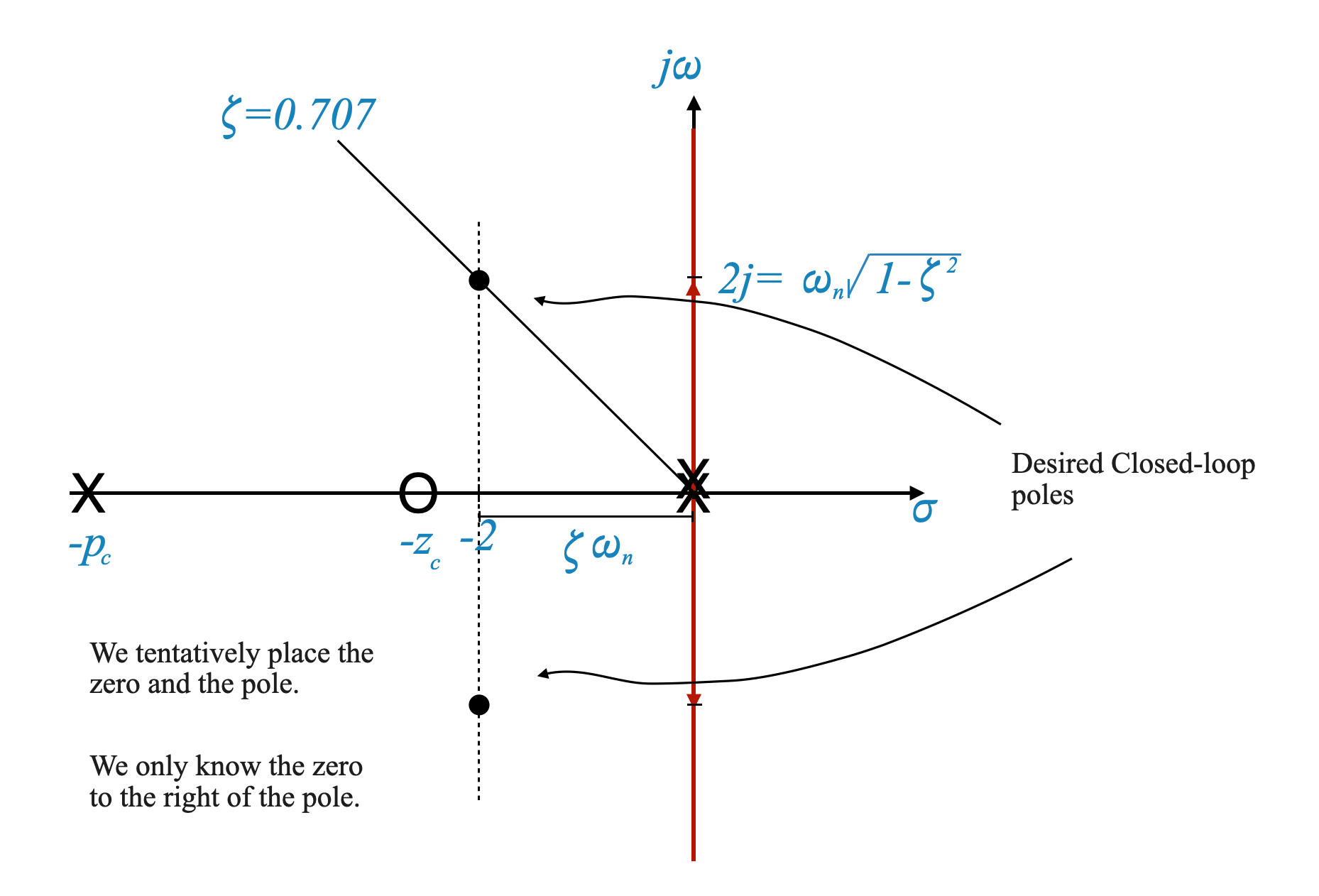
Designing the Phase Lead Compensator: Placing the Zero and the Pole
Step 1: Initial Placement of Zero and Pole on the s-plane
Start by placing the zero ($ z_c \() and the pole (\) p_c $) of the compensator tentatively on the s-plane. This initial placement doesn’t have to be exact; it’s a starting point for fine-tuning.
Zero ($ z_c $): Place it closer to the imaginary axis.
Pole ($ p_c $): Place it further left from the zero on the real axis.
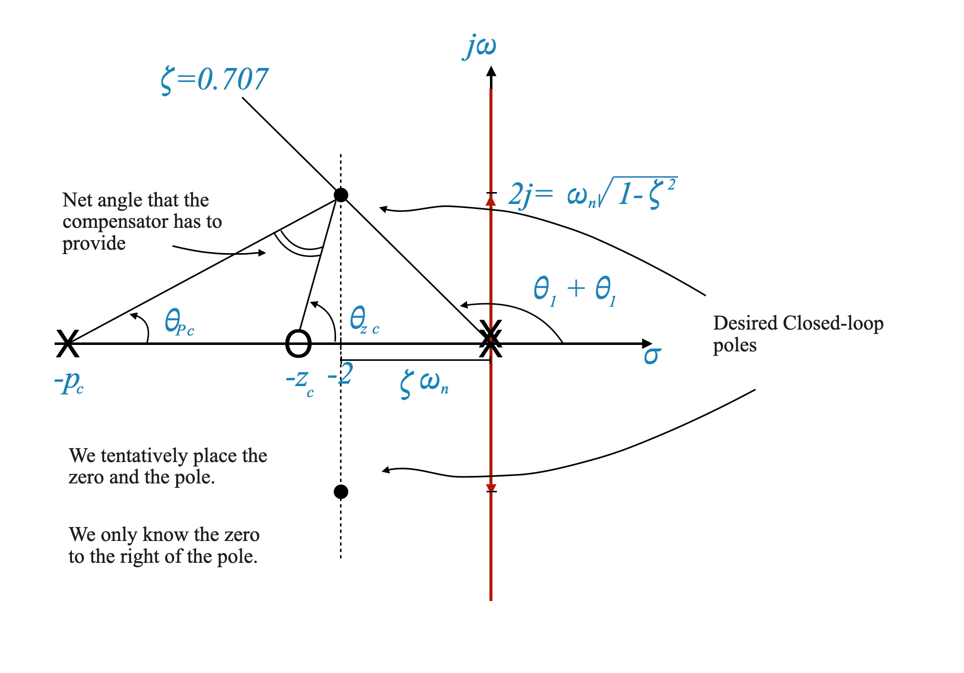
Step 2: Adjusting for Angle Criterion
To ensure the system’s closed-loop response meets our requirements, the root locus must pass through the desired closed-loop pole locations. This requires satisfying the angle criterion at these points.
Understanding the Angle Criterion:
The angle criterion states that the sum of phase angles from all poles and zeros to a point on the s-plane must equal an odd multiple of 180 degrees for the point to be on the root locus.
For a lead compensator, the important angles are those contributed by the compensator’s zero ($ {z_c} \() and pole (\){p_c} \(), and the angle from the plant's poles (\) _1 $).
Calculating the Angle Contributions:
We need to find the angles $ {z_c} $ and $ {p_c} $ such that they fulfill the equation:
Here, $ {z_c} $ and $ {p_c} $ are the angles from the compensator’s zero and pole to the desired closed-loop pole location, respectively, and $ 2_1 $ is the contribution from the plant’s poles.
Step-by-Step Guide to Compensator Design with Root Locus
Understanding the Role of Poles and Angles
Starting Point: We know the plant’s poles, hence we can determine $ _1 $, the angle contribution from these poles to any point in the s-plane.
Desired Closed-Loop Poles: In our example, they are at $ -2 j2 $. This gives us a reference for determining the necessary angle contributions from the compensator.
Calculating the Compensator’s Contribution
Net Angle Contribution: The compensator must provide a net angle $ {z_c} - {p_c} $, where $ {z_c} $ and $ {p_c} $ are the angles from the compensator’s zero and pole to the desired closed-loop poles.
General Strategy: Typically, we choose a location for the zero and then calculate where the pole should be to meet the angle condition.
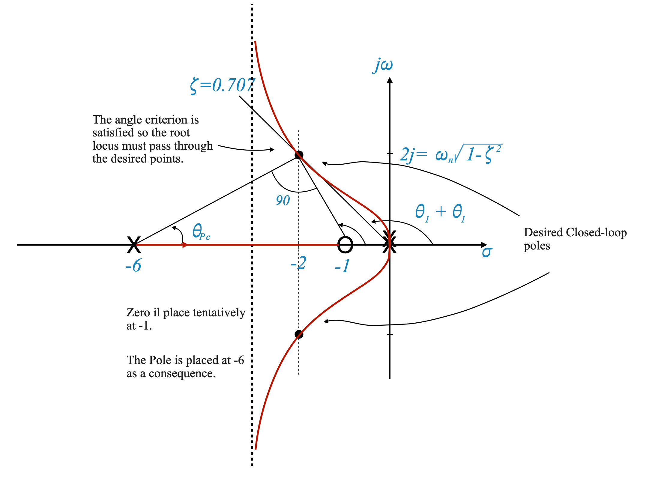
Example Calculation:
Place the zero at -1 on the real axis of the s-plane.
The resulting root locus shows that the angle condition is met (we have designed it to meet it), and the locus goes through the desired closed-loop poles.
Evaluating the Design
Dominance Condition: Even though the angle condition is satisfied, we must ensure that the dominance condition is also met. This means the designed system’s behavior should closely match the expected behavior from a second-order system with the given $ $.
Problem with Third Pole: In our example, the third pole moves close to the zero, potentially affecting the system’s overshoot and not satisfying the dominance condition.
Calculating the Third Pole and Verifying Dominance
Magnitude Criterion: Use the magnitude criterion to calculate the value of $ K $ corresponding to the desired closed-loop poles. In this case, $ K = 16 $.
Finding the Third Pole: With $ K = 16 $, locate the third pole and verify if the dominance condition is met.
Simulation: If the dominance condition is not met, simulate the system’s response to evaluate the influence of the third pole.
Guidelines for Placing the Zero
Preferred Location: Ideally, place the zero to the left of the desired complex conjugate closed-loop poles. This ensures that the third pole lies to the left of the desired poles, satisfying the dominance condition. This is because the root locus branch will end at that zero.
Exceptions: Sometimes, this ideal placement isn’t possible. In such cases, as with our 90° net angle contribution, we may need to place the zero to the right.
Solving for \(K\)
To solve for the gain $ K $ in our control system example, where the zero of the compensator $ z_c $ is at -1 and the pole $ p_c $ is at -6, we follow the steps laid out earlier. We need to calculate $ K $ such that the magnitude condition is satisfied at the desired closed-loop poles $ -2 j2 $.
Given:
Desired closed-loop poles: $ -2 j2 $
Zero $ z_c = -1 $
Pole $ p_c = -6 $
The open-loop transfer function $ G(s) $ is:
\[ D(s)G(s) = \frac{K \cdot (s + z_c)}{s^2 \cdot (s + p_c)} \]
Substituting $ z_c = -1 $ and $ p_c = -6 $ into the transfer function, we get:
\[ D(s)G(s) = \frac{K \cdot (s + 1)}{s^2 \cdot (s + 6)} \]
Applying the Magnitude Condition
Now, we apply the magnitude condition at one of the desired closed-loop poles, say $ s = -2 + j2 $:
\[ \frac{K \cdot \text{Magnitude of Numerator}}{\text{Magnitude of Denominator}} = \frac{8(4.47)}{2.23} = 16\]
Balancing Angle Conditions and Noise Attenuation in Compensator Design
In the design of a compensator, particularly a phase lead compensator, a crucial aspect to consider is the relationship between the compensator’s pole and zero. This relationship is not just a matter of meeting geometric conditions for angle requirements but also plays an important role in noise attenuation, especially for high-frequency signals.
The Role of Pole-Zero Ratio
Geometric Considerations for Angle Conditions:
The placement of the pole and zero on the s-plane is initially guided by the need to satisfy the angle condition of the root locus method.
This condition ensures that the compensator effectively alters the system’s root locus to achieve desired transient response characteristics.
Noise Filtering Aspect:
Apart from meeting angle conditions, the pole in the compensator acts as a filter for high-frequency noise.
The location of the pole relative to the zero significantly impacts the compensator’s ability to attenuate high-frequency components.
Ideal Ratio Between Pole and Zero
Factor of 10 for Attenuation:
It is generally recommended that the ratio between the zero and the pole be around 10. This ratio has been found to provide effective high-frequency attenuation.
For instance, if the zero is placed at -1 on the real axis, a corresponding pole at -10 can offer a good balance between angle condition satisfaction and noise reduction.
Balancing Design Objectives
Trade-offs in Design:
Often, control system designers face a trade-off between strictly adhering to the angle conditions for desired transient performance and positioning the pole for optimal high-frequency noise attenuation.
This balance is critical in ensuring that the compensator not only improves system response but also maintains robustness against high-frequency disturbances.
Finding the third pole
To calculate the location of the third pole in a control system where a phase lead compensator has been added, and the gain $ K $ has been determined, we can follow these steps:
Open-Loop Transfer Function: Recall the open-loop transfer function with the compensator: \[ D(s)G(s) = \frac{K \cdot (s + z_c)}{s^2 \cdot (s + p_c)} \] where $ z_c $ is the zero and $ p_c $ is the pole of the compensator.
Substitute Known Values: Substitute the known values for $ K $, $ z_c $, and $ p_c $ into the open-loop transfer function.
Root Locus Method: To find the location of the third pole, you can use the root locus method. This involves plotting the root locus of the open-loop transfer function and identifying where the third pole lies based on the value of $ K $.
Analytical Approach: Alternatively, for an analytical approach, you can set up the characteristic equation of the closed-loop system, which is: \[ 1 + G(s)H(s) = 0 \] Solving this equation will give you the poles of the closed-loop system.
Solving the Characteristic Equation: The characteristic equation will be a cubic equation in $ s $ (since the original system is second-order and the compensator adds one order). Solving this cubic equation will give you three solutions, corresponding to the three poles of the closed-loop system.
Identifying the Third Pole: Two of these poles will be the desired closed-loop poles (e.g., $ -2 j2 $ in our example). The third solution will be the additional pole introduced by the compensator.
Practical Considerations
Computational Tools: Solving the cubic equation analytically can be complex. It’s often more practical to use computational tools like MATLAB or Python, which can efficiently compute the roots of polynomial equations.
Dominance of Poles: Once you find the third pole, you should check its dominance in the system’s response. If it’s far left in the s-plane, its effect on the system’s transient response might be negligible. If it’s closer to the imaginary axis, it might significantly influence the system’s behavior.
import numpy as np# Coefficients of the cubic equationcoefficients = [1, 6, 16, 16]# Finding the rootsroots = np.roots(coefficients)# Display the rootsprint("The poles of the system are:", roots)
The poles of the system are: [-2.+2.j -2.-2.j -2.+0.j]
import numpy as npimport matplotlib.pyplot as pltimport control as ctlfrom ipywidgets import interact, FloatSliderdef calculate_settling_time(T, yout, tol=0.02):# Settling time is the time at which the response remains within a certain tolerance settled_value = yout[-1] lower_bound = settled_value * (1- tol) upper_bound = settled_value * (1+ tol) within_tol = np.where((yout >= lower_bound) & (yout <= upper_bound))[0]if within_tol.size ==0:return np.nan # Return NaN if the system never settlesreturn T[within_tol[0]]def calculate_steady_state_error(system_type, G, K, time_span): G_closed_loop = ctl.feedback(K * G)if system_type =='step':# Steady-state error for step input (Type 0 system) T, yout = ctl.step_response(G_closed_loop, T=np.linspace(0, time_span[-1], 500)) steady_state_val = yout[-1]return1- steady_state_valelif system_type =='ramp':# Steady-state error for ramp input (Type 1 system) Kv = ctl.dcgain(G_closed_loop * ctl.TransferFunction([1, 0], [1]))return1/ Kv if Kv !=0else np.infelse:return np.nan# def plot_step_response(G, K, time_span):# G_closed_loop = ctl.feedback(K * G)# T, yout = ctl.step_response(G_closed_loop, T=np.linspace(0, time_span[-1], 500))# plt.plot(T, yout)# settling_time = calculate_settling_time(T, yout)# steady_state_error = calculate_steady_state_error('step', G, K, time_span)# plt.title(f'Step Response for Gain K={K}\nSettling Time: {settling_time:.2f}, Steady-State Error: {steady_state_error:.2f}')# plt.xlabel('Time')# plt.ylabel('Amplitude')# plt.grid(True)# def plot_ramp_response(G, K, time_span):# G_closed_loop = ctl.feedback(K * G)# T, yout = ctl.forced_response(G_closed_loop, T=time_span, U=time_span)# plt.plot(T, yout)# steady_state_error = calculate_steady_state_error('ramp', G, K, time_span)# plt.title(f'Ramp Response for Gain K={K}\nSteady-State Error: {steady_state_error:.2f}')# plt.xlabel('Time')# plt.ylabel('Amplitude')# plt.grid(True)def plot_root_locus_with_gain(K, numerator, denominator):# Define the transfer function G(s) G = ctl.TransferFunction(numerator, denominator)# Calculate the closed-loop transfer function for the given gain G_closed_loop = ctl.feedback(K * G)# Find the poles for the specific gain poles = ctl.pole(G_closed_loop)# Plot the root locus plt.figure(figsize=(10, 6)) ctl.root_locus(G, plot=True)# Plot the poles for the specific gain plt.plot(np.real(poles), np.imag(poles), 'ro', markersize=10, label=f'Poles for K={K}')# Enhance plot plt.xlabel('Real Axis') plt.ylabel('Imaginary Axis') plt.title(f'Root Locus of G(s) with Poles for Gain K={K}') plt.grid(True) plt.legend() plt.show()def plot_all(K):# Define the transfer function D(s)G(s) numerator = [1, 1* zc] # 16s+16 denominator = [1, 6, 0, 0] # s^3 + 6s^2 G = ctl.TransferFunction(numerator, denominator)# Time span for the responses time_span = np.linspace(0, 10, 1000)# Plot Root Locus plot_root_locus_with_gain(K, numerator, denominator)# # Plot Step Response# plt.figure(figsize=(10, 4))# plot_step_response(G, K, time_span)# plt.show()# # Plot Ramp Response# plt.figure(figsize=(10, 4))# plot_ramp_response(G, K, time_span)# plt.show()zc =1# Zero of the compensatorinteract(plot_all, K=FloatSlider(value=16, min=0, max=50, step=0.5, description='Gain K:'))
<function __main__.plot_all(K)>
import numpy as npimport matplotlib.pyplot as pltimport control as ctl# Define system parametersK =1# This is one to have K to vary in the plot. We need to click on the value of gain 16.zc =1# Zero of the compensatorpc =6# Pole of the compensator# Define the transfer functionnumerator = [K, K * zc] # 16s+16denominator = [1, 6, 0, 0] # s^3 + 6s^2system = ctl.tf(numerator, denominator)# Plot the root locusctl.rlocus(system)plt.show()# Use the plot to find the third pole at the specific gain K
Interactive Learning
Consider designing a phase lead compensator for a system where transient performance is as crucial as noise reduction. The choice of pole and zero locations would need to:
Satisfy Angle Conditions: Ensure that the root locus passes through desired closed-loop pole locations for the required transient response.
Filter High-Frequency Noise: Position the pole such that it effectively filters out undesirable high-frequency components, without adversely impacting the transient response.
Interactive Exercise: Students can engage in an exercise using a software tool like MATLAB or Python to experiment with different pole-zero ratios. Observing how these adjustments affect both the transient response and noise attenuation will provide practical insights into the trade-offs involved in compensator design.
Steady state requirements
Given that we have a type-2 system this is not a concern, certainly not for steps and ramps. If acceleration error is to be calculated this can be done from:
\[ D(s)G(s) = \frac{K \cdot (s + z_c)}{s^2 \cdot (s + p_c)} = \frac{16 \cdot (s + 1)}{s^2 \cdot (s + 6)} \]
and hence, the acceleration constant is:
\[
K_a = \frac{16}{6}
\]
and the corresponding acceleration error is:
\[
e_{ss} = \frac{6}{16} radians
\]
This is a finite value and most likely acceptable. Following acceleration is difficult and typically we are satisfied with step and ramp inputs.
Phase Lag Compensation
In this part, we’ll delve into the concept of phase lag compensation. Unlike phase lead compensators that are designed to improve transient performance, phase lag compensators are primarily used to enhance steady-state accuracy.
The Phase Lag Network Model
Transfer Function of Phase Lag Compensator
The transfer function for a phase lag compensator is generally given by:
\[ D(s) = \frac{s + z_c}{s + p_c} \]
Where: - $ z_c $ is the zero of the compensator. - $ p_c $ is the pole of the compensator.
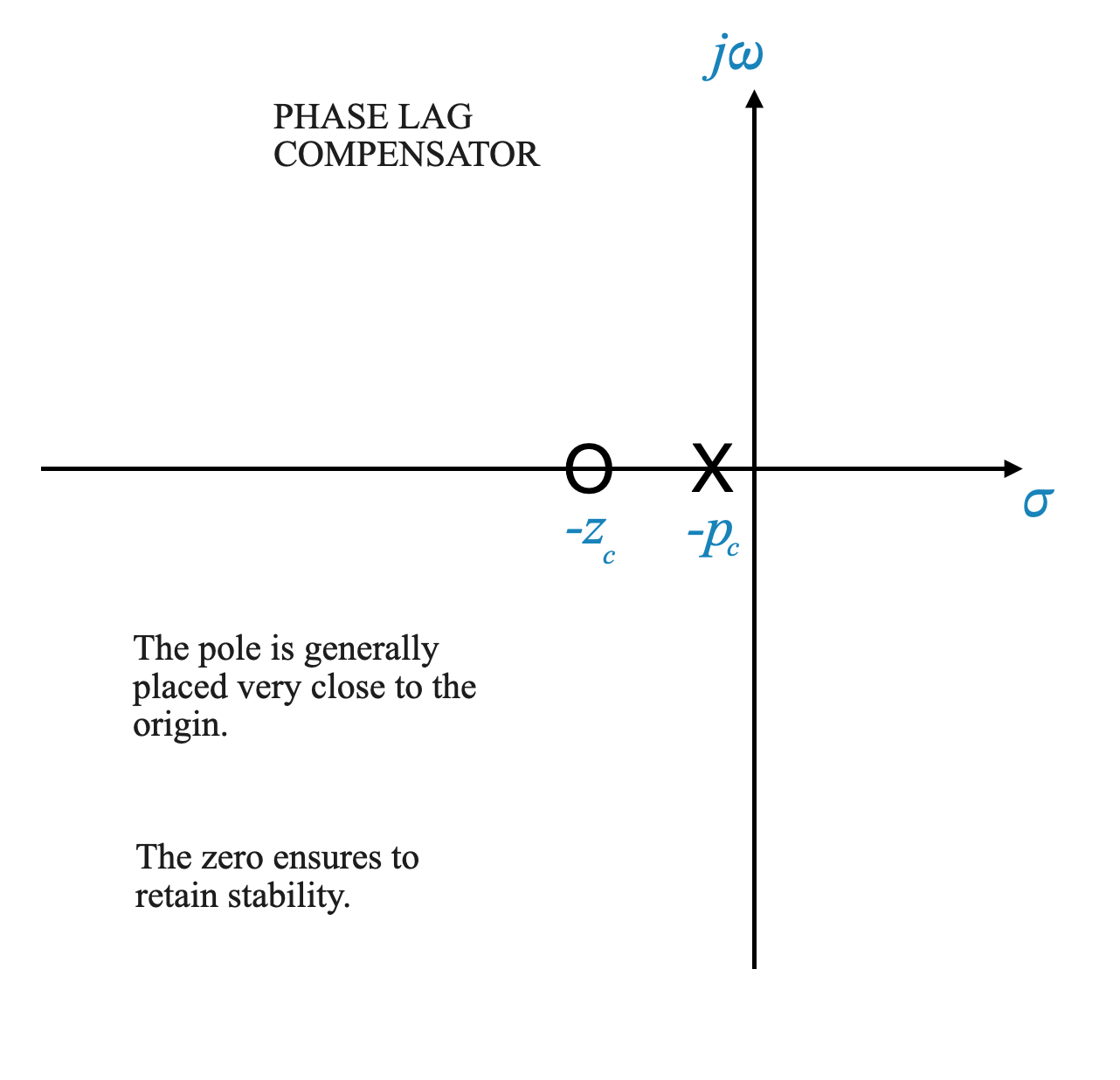
Pole-Zero Configuration
In a phase lag compensator, the pole is usually placed close to the origin but not necessarily at it. Placing a pole at the origin makes it a Proportional-Integral (PI) controller.
The zero ($ z_c \() is positioned close to the pole (\) p_c $), which is essential for maintaining system stability. Otherwise, the presence the pole at the origin might destabilise the system.
Choosing Between Phase Lag and Phase Lead Compensators
Decision Criteria
Transient Performance Requirements:
If the uncompensated system, via a gain adjustment, meets the transient performance requirements, then a phase lag compensator can be considered.
If not, and you are not able to choose a gain that meets the transient performance requirements, and if there’s a need to pull the root locus to the left, a phase lead compensator is more appropriate.
The gain of the uncompensated system is a critical factor. By adjusting this gain, you might meet the transient performance requirements without needing additional compensation.
Steady-State Accuracy:
For improving steady-state accuracy, particularly in type-1 or type-0 systems, a phase lag compensator is a suitable choice. Using a lag compensator with a type-2 system is very difficult due to the unstabilising effects.
Using a lag compensator is similar to adding an integrator to improve the steady state performance. The pole and zero are chosen so that the transient performance are not deteriorated. Having the zero as close as possible to the pole means that we want to reduce the effect that the compensator might have on the transient.
Example: Applying Phase Lag Compensation
System Model
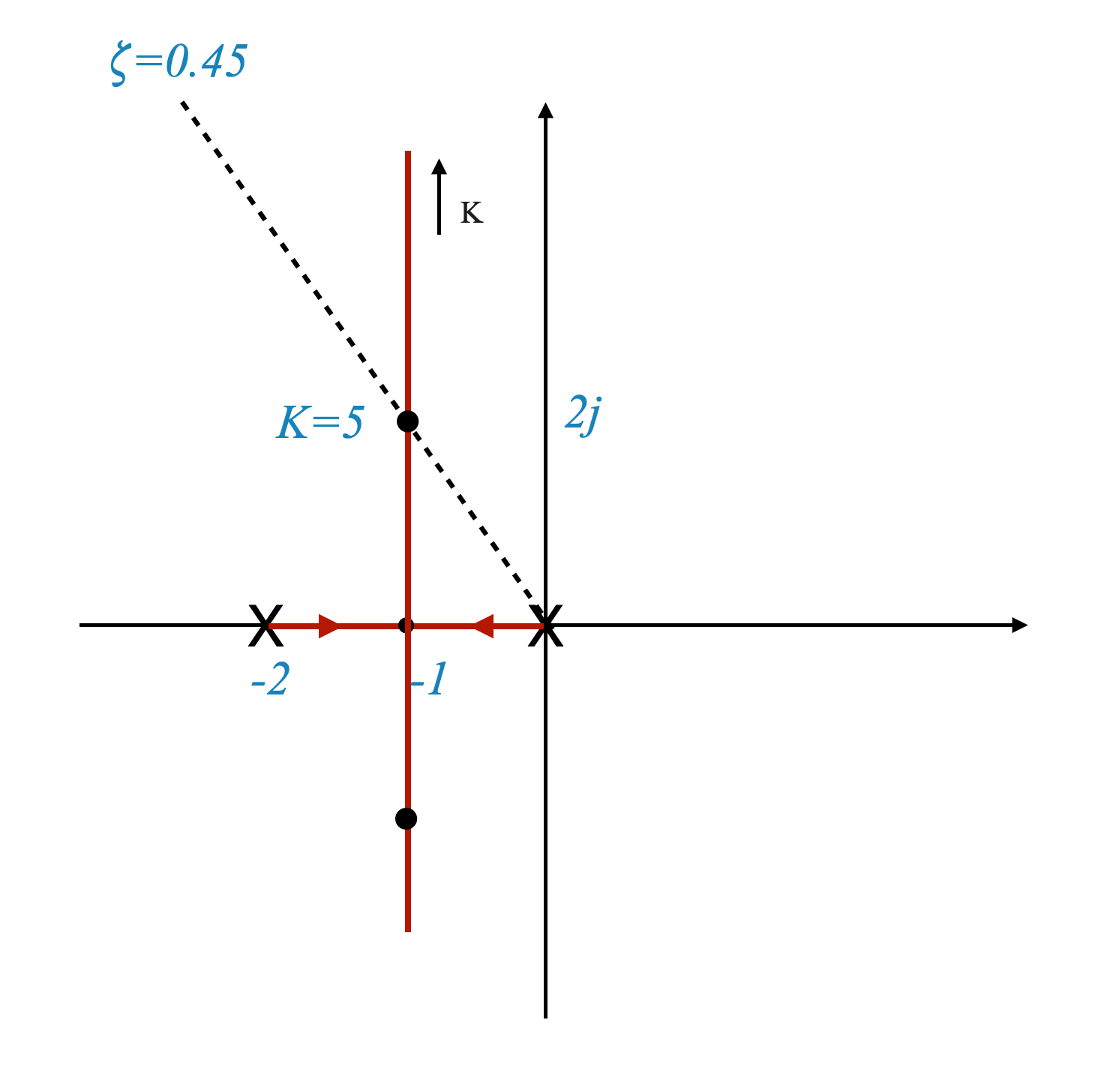
Let’s consider a type-1 system represented by:
\[ G(s) = \frac{K}{s(s + 2)} \]
This model could represent a motor servo system for position tracking.
In our control system example, let’s begin by assessing the uncompensated system’s performance. A key parameter in this assessment is the velocity error constant, denoted as $ K_v $. For our system, $ K_v $ is calculated as follows:
\[ K_v = \frac{K}{2} \]
$ K_v $ is a measure of the system’s ability to track ramp inputs. A higher $ K_v $ implies better tracking performance for such inputs.
Desired Closed-Loop Pole Locations
Calculating Pole Locations for Given Damping Ratio
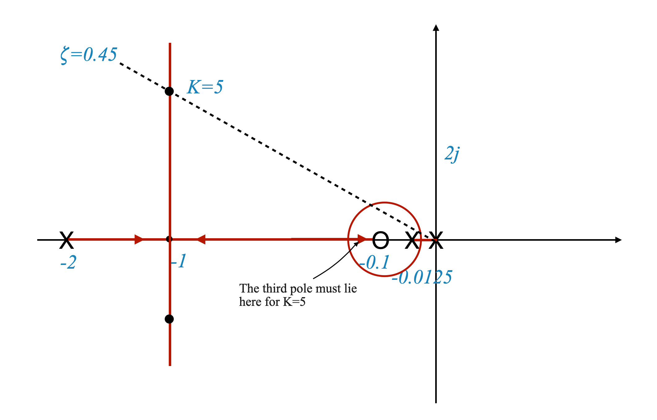
For a damping ratio ($ $) of 0.45, the closed-loop poles are located at $ -1 2j $.
This calculation is based on standard second-order system dynamics where the pole locations are determined by the damping ratio and the natural frequency.
The location of these poles in the s-plane directly affects the transient behavior of the system, including aspects like overshoot and settling time.
Assessing System Performance at $ K = 5 $
Determining When Desired Poles Are Achievable
Figure: root locus plot that shows how varying $ K $ affects the pole locations.
By examining the root locus plot, we can identify that the desired closed-loop poles at $ -1 2j $ are obtainable when the gain $ K $ is set to 5.
Steady-State Accuracy
When $ K = 5 $, the velocity error constant is:
\[ K_v = \frac{K}{2} = \frac{5}{2} = 2.5 \]
However, this value of $ K_v $ is less than the required 20 for adequate steady-state performance.
The Objective of Phase Lag Compensation
Boosting $ K_v $ to Meet Steady-State Requirements
The primary goal of introducing a phase lag compensator in this scenario is to increase $ K_v $ to meet the steady-state requirement of 20.
This needs to be achieved while ensuring that the compensated root locus plot passes through the desired closed-loop poles at $ -1 2j $.
Balancing Steady-State and Transient Performance
The challenge lies in boosting $ K_v $ without adversely affecting the transient performance, which is indicated by the closed-loop pole locations.
Meeting the transient requirements
To accomplish our desired outcome, we will position both the zero and the pole of the compensator near the origin. The goal here is to ensure that their combined contribution to the phase angle of the system is minimal, ideally within a range of 1 to 5 degrees. By doing so, we can effectively ensure that these elements have a negligible impact on the system’s original root locus plot. This strategic placement is crucial for maintaining the original characteristics of the system while implementing the phase lag compensator.
this means that we can use the ratio \(\frac{z_c}{p_c}\) to improve our velocity constant.
More specifically, for \(K=5\) (note that for the same reason why the zero and pole do not disturb the transient, they also do not change much the value of the root locus gain, the boost that we need is \(\frac{z_c}{p_c}=8\).
This helps us define the relationship between the zero and the pole of the compensator.
Placing the pole and zero
We start from placing the zero at \(z_c = -0.1\) (this comes from the dominance condition as we will see soon).
The pole hence is located at: \(p_c = \frac{-0.1}{8}=0.0125\)
The root locus is (this is not too scale to highlight the relationships):
Dominance Condition
It is possible to verify that the third pole must be real, and hence very close to the zero. This means that the dominance condition is satisfied (even though it is close to the imaginary axis). If the third pole is not close enough we can make an adjustment to the zero/pole locations to move it closer to the zero. This is typically done using software.
Simulations
Finally through simulation we can verify the full performance (transient and steady-state) of the system.
Lag-Lead Compensation
In concluding our discussion on control system compensators, let’s consider how to choose between different types of compensators based on the performance of the uncompensated system. Here, by ‘uncompensated,’ we mean a system where only gain adjustments are permissible.
Decision Making for Compensator Type
When to Choose a Lag Compensator:
If the transient performance of the uncompensated system is satisfactory, then a lag compensator is a suitable choice.
The primary role of the lag compensator here is to enhance steady-state performance without significantly affecting the transient response.
Choosing a Lead Compensator:
If the transient performance is unsatisfactory, a lead compensator is the way to go.
The lead compensator is designed to improve transient performance. After implementing it, you should re-evaluate to see if steady-state requirements are met.
Addressing Both Transient and Steady-State Performance
Scenario: What if, after designing a phase lead compensator, both transient performance is not satisfactory, and steady-state requirements are unmet?
Solution: In such cases, consider using a lag-lead compensator. This involves first designing a lead compensator to address transient performance and then evaluating steady-state performance.
The Standard Final Procedure
Evaluate the Open-Loop System:
Carefully investigate the open-loop system with gain adjustments to assess transient performance.
Design Process:
If transient performance is adequate, opt for a lag compensator.
If transient performance is inadequate, design a lead compensator to rectify this.
After implementing the lead compensator, check the steady-state error. If it’s satisfactory, your design is complete.
Incorporating Lag Compensator if Necessary:
If steady-state performance is still lacking, treat the lead-compensated system as ‘uncompensated’ for the purpose of designing a phase lag compensator.
The lag compensator, in this case, won’t disturb the transient improvements made by the lead compensator.
Final Design Choices
Your final design choice can be a lead, lag, or a combination of lead-lag compensators, depending on the system’s requirements.
Operational Amplifier (Op-Amp) realizations for both lead-lag and lag-lead compensators have been discussed, allowing for practical implementation and parameter adjustments.
Conclusion: The design and selection of compensators depend on both the transient and steady-state performance requirements of your system. The decision-making process involves a careful evaluation of the system’s current performance and the objectives you aim to achieve with compensation.
Note for Instructor: Encourage students to analyze different system scenarios and decide on the type of compensator needed. Practical exercises involving Op-Amp circuit design for lead-lag and lag-lead compensators can be very beneficial for understanding these concepts.