Introduction to Control Systems

In this notebook, we will explore the fundamental concepts of control systems and the various modes of control, including proportional control, integral control, and derivative control.

In a control system, we have a basic feedback structure consisting of several components:

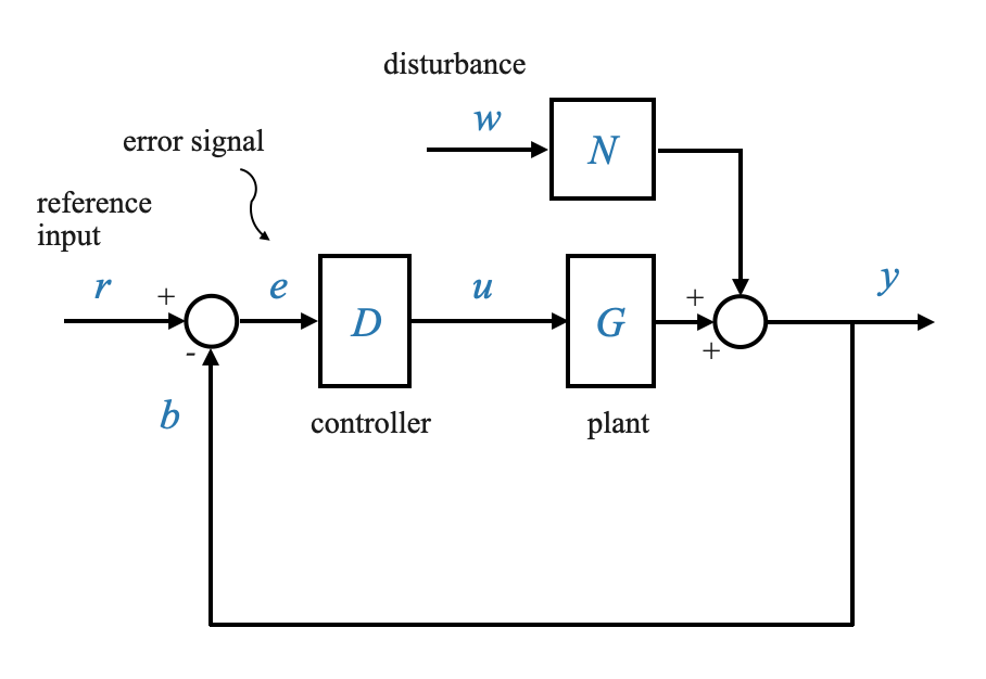
For simplicity we are considering a unity-feedback system, and hence we focus on the system error $e$ directly.

• \(G(s)\): This represents the plant, which we will, for simplification, denote as SG.
• \(D\): The transfer function of our controller.
• \(N\): A model capturing disturbances acting on the system.
• \(y\): Our controlled variable.
• \(y_r\): The command or reference signal.
• \(e = y_r - y\): The error signal

Notes: - Unity feedback so \(e = r-y\), whereas if it was through a sensor we would have had \(\hat{e}\).

• Now, let’s focus on the controller, denoted as \(D\). Until now, the most basic type of controller we’ve utilized is an amplifier. We have explored amplifiers with different gains in a variety of industrial contexts in this course. However, as we observed in our previous discussion, an amplifier alone might not meet all our performance goals. There’s an inherent conflict in performance objectives. For instance, enhancing the gain of the amplifier improves certain performance characteristics of the system, but simultaneously, it can detrimentally impact other crucial aspects.

• We also need to keep in mind that we do not need to constrain the shape of \(D(s)\).

Historically there were hardware limitations (controllers had to be hydraulic, pneumatic or electrical).

With the advent of digital technology, virtually any function can be realized through a digital computer, removing the limitations of hardware-based control systems.

Proportional Control (P-Control)

Proportional control is one of the simplest control modes. The control signal $u$ in proportional control is given by:

\[ u = K_c \cdot e \]

Where \(K_c\) is the controller gain.

In the Laplace domain:

\[ U(s) = K_c \cdot E(s) \]

Proportional - Integral Control (PI-Control)

Proportional-Integral control, often known as PI control, introduces integral action to improve control performance.

The control signal \(u\) in integral control is given by:

\[ u = K_c \cdot \big( e + \frac{1}{T_I} \int e dt \big) \]

It is composed of two components, one which is proportional to the error, and one that is proportional to the integral of the error.

In the Laplace domain:

\[ u = K_c \cdot \big( 1 + \frac{1}{T_I s}\big)E(s) \]

Sometime also written as:

\[ u = \big( K_c + \frac{K_I}{s}\big)E(s) \]

Where: - \(K_I\) is called integral gain - \(K_c\) is called controller gain - \(T_I\) is the integral time or reset time.

We’ll explore the benefits of integral control and its application in control systems.

Proportional-Derivative Control (PD-Control)

Proportional-Derivative control, often known as PD control, introduces derivative action to control systems.

The control signal \(u\) in derivative control is given by:

\[ u = K_c \big(e + T_D \dot{e}\big ) \]

In the Laplace domain:

\[ U(s) = K_c \big(1 + T_D s\big )E(s) \]

Where \(T_D\) is the derivative time or rate time.

Sometime also written as:

\[ u = \big( K_c + K_D s\big)E(s) \]

Where \(K_D\) is called derivative gain.

We’ll examine the role of derivative control and its impact on control system performance.

PID Control

PID control combines proportional, integral, and derivative actions in a single controller. The control signal \(u\) in PID control is given by:

\[ u = K_c \cdot (e + \frac{1}{T_I} \int e dt + T_D \cdot \frac{de}{dt}) \]

\[ U(s) = K_c \big(1+\frac{1}{T_I s} + T_Ds\big)E(s) \]

Sometime written also as:

\[ U(s) = \big(K_c+\frac{K_I}{s} + K_Ds\big)E(s) \]

Often used as first attempt before attemping different methods if the PID does not work.

Example: Temperature Control System

Consider a temperature control system designed to maintain a chamber’s temperature at a prescribed level. This system serves as an excellent illustration of proportional control.

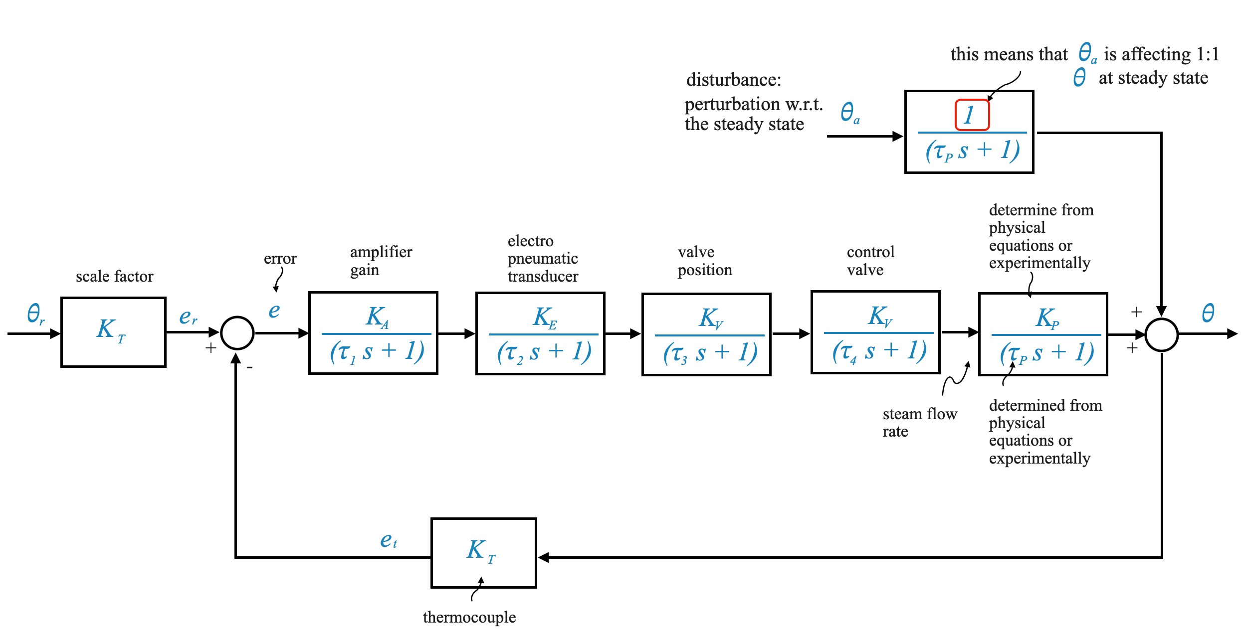
• System Description: We consider a temperature control system, which is a chamber where the temperature needs to be maintained at a specific level \(\theta_r\). The disturbance variable (ambient temperature) in this system is denoted as \(\theta_a\), and \(\theta\) represente the temperature of the chamber.

• Application Context: This system can be likened to a testing chamber for electronic equipment, where the temperature needs to be regulated for testing the components under different thermal conditions.

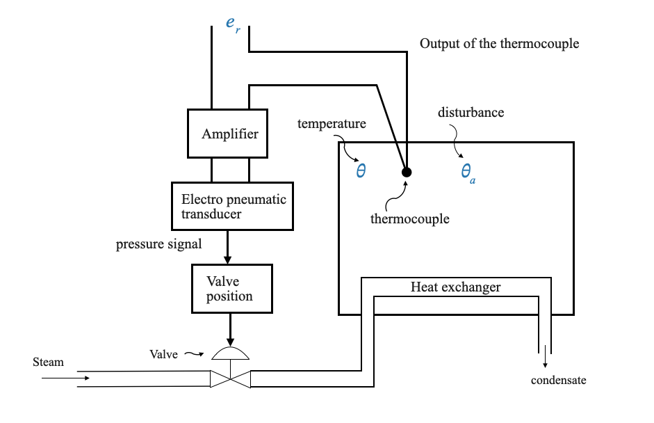
System Components: - Chamber Temperature (\(\theta\)): The primary variable to be regulated. - Disturbance Variable (\(\theta_a\)): External factors influencing the chamber temperature, such as ambient temperature. - Thermocouple: A sensor used to measure the chamber’s temperature. - Electropneumatic Transducer: Converts the electrical signal to a pressure signal. - Valve Positioner: Adjusts a valve to control steam flow, thereby regulating the chamber’s temperature. - Heat Exchanger: Facilitates the heating of the air inside the chamber.

Operation: -The desired temperature (\(\theta_r\)) is set and compared with the actual temperature (θ). - The thermocouple generates an electrical signal proportional to the temperature difference. - This signal is amplified and used to adjust the valve position, controlling the steam flow and, consequently, the temperature.

Control Requirements

• Objective: Maintain the chamber temperature at a regulated value, \(\theta_r\).
• Sensing the Temperature: A thermocouple is used as a sensor to measure the chamber’s temperature.
• Error Calculation: The sensor output, denoted as \(e_t\), is compared with a reference value \(e_r\) (proportional to \(\theta_r\)) to calculate the error signal \(e\).

Contoller and actuators

• Amplifier as Controller: The output of the amplifier, based on the error signal, is used to control the Electropneumatic transducer, which in turn generates a pressure signal.
• Valve Positioner: This device adjusts the valve based on the pressure signal, controlling the steam flow and thus the temperature in the chamber.

Disturbances

• Sources of Disturbance: Changes in environmental temperature or command signal variations are the primary disturbances.
• System’s Response: The control system adjusts the steam flow rate to restore equilibrium in response to disturbances.

Using a Proportional Proportional

We analyze how effective proportional control is in maintaining the desired temperature in the presence of disturbances.

🤔 Popup Question: What happens to the error signal \(e\) when the chamber temperature \(\theta\) is equal to the setpoint \(\theta_r\)?

Answer: The error signal \(e\) becomes zero, indicating no discrepancy between the desired and actual temperature.

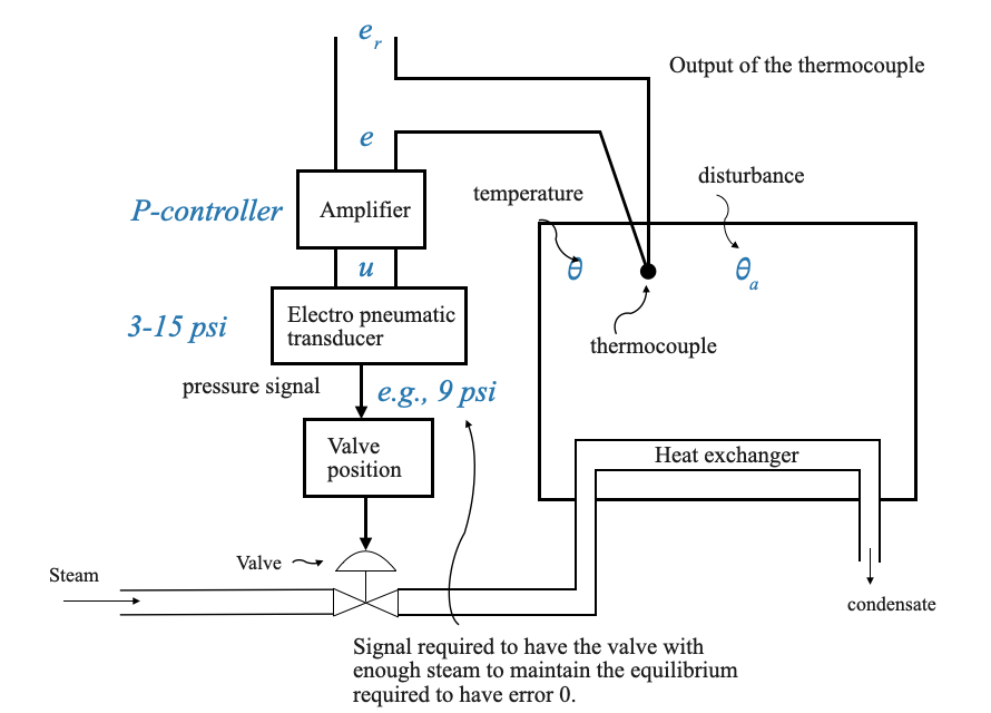
In the state of equilibrium, both the error signal and the control signal are null. The initial adjustment of the Electropneumatic transducer within the valve positioner upholds the heat equilibrium. This adjustment additionally compensates for any heat loss to the surroundings, provided that the ambient temperature remains constant.

What happens if there are disturbances?

Perturbations from the equilibrium position can be created by - Change in the environment - Change in the command signal

When this happens, we have an error signal \(e\) and a corresponding control signal \(u\) that needs to readjust the steam flow rate to get to a new equilibrium.

Modeling the Temperature Control System

• Mathematical Model: We can model the chamber as a first-order system with a transfer function

\[ \frac{K_p}{\tau_p s + 1} \]

where \(K_p\) is the process gain and \(\tau_p\) is the time constant.

• Disturbance: Changes in the environmental temperature (\(\theta_a\)) can perturb the system from its equilibrium.

We can hence model the disturbance influence as a first-order system with a transfer function

\[ \frac{1}{\tau_p s + 1} \]

Setting \(K\) as 1 implies that we are assuming a direct, one-to-one impact of $ _a $ on $ $ at the steady state. If an experimental assessment reveals a variance from this assumption, an appropriate constant can be introduced to account for the difference.

When we consider dynamical models we always consider with respect to the steady state. The total ambient temperature is not \(\theta_a\), which is the perturbation of the ambient temperature from the point of equilibrium.

Block Diagram

We can then write the block diagram of the temperature control system, illustrating the relationship between the control signal, the plant, and the output.

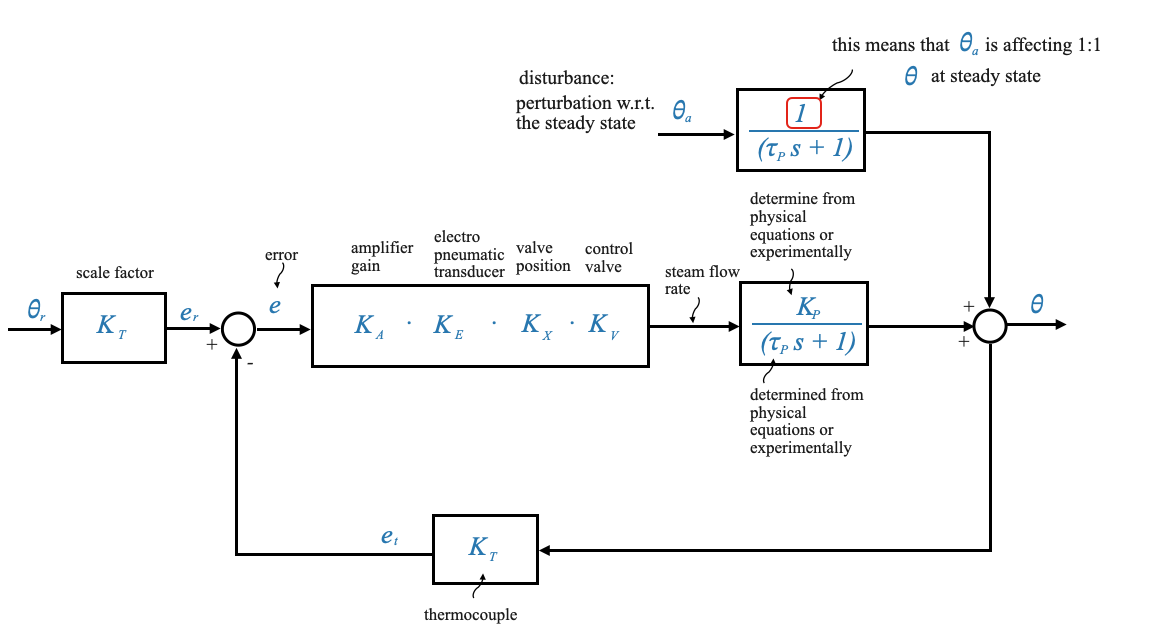
In the example of the temperature control system, we are looking at a Proportional (P) controller where various gains are multiplied together. Let’s break down these gains and their units to understand the overall unit of the proportional controller in this context.

Breakdown of the Gains and Their Units

1. Amplifier Gain (\(K_A\)): This gain typically has the unit of volts per volt (V/V), as it relates the output voltage to the input voltage of the amplifier.

2. Electropneumatic Transducer Gain (\(K_e\)): This gain converts the electrical signal (voltage) to a pneumatic signal (pressure).

3. Valve Positioner Gain (\(K_x\)): This relates the pneumatic pressure signal to the mechanical position of the valve. Its unit could be dimensionless, representing the ratio of the valve stem displacement to the input pressure signal (e.g., mm/psi or mm/bar).

4. Control Valve Gain (\(K_v\)): This gain describes how the position of the valve affects the flow rate of the steam. The unit could be in terms of steam flow rate per unit displacement, such as cubic meters per hour per millimeter (m³/h/mm).

Calculation of Proportional Controller’s Overall Gain

When these gains are multiplied together, the resulting unit of the proportional controller’s overall gain (\(K\)) will be a composite of all these individual units. In the given scenario, the units would multiply as follows:

\[ K = K_A \times K_e \times K_x \times K_v \]

So, for example, the unit of \(K\) would be:

\[ \text{V/V} \times \text{psi/V} \times \text{(mm/psi)} \times \text{(m³/h/mm)} \]

When simplified, this gives us:

\[ \text{m³/h/V} \]

Interpretation

The resulting unit of m³/h/V indicates that the controller’s output, in terms of steam flow rate (m³/h), is proportional to the voltage input to the system. This reflects the essence of a proportional controller, where the output is directly proportional to the error signal, which, in this case, is represented in voltage.

This detailed understanding of units is crucial for designing and tuning control systems, ensuring that the controller operates within the desired range and effectively manages the plant it is controlling.

Components as zero-order systems

We have simplified our model by treating all these components as zero-order systems, disregarding their inherent dynamics. It’s important to remember that these components do possess dynamic characteristics.

Characterizing them as zero-order systems implies an assumption of instantaneous response, which is not possible for any physical system. Nonetheless, this simplification is made because the time constants of these individual components are considerably small compared to the plant’s time constant, $ _p $.

Understanding the Impact of Disturbance (\(\theta_a\))

With reference to the physical drawing shown above, consider an increase in the ambient temperature (\(\theta_a\)). Intuitively, if the external temperature rises, the outflow of heat from the system will reduce, leading to an increase in the chamber’s temperature.

Given this understanding, we’ll consider the effect of the disturbance \(\theta_a\) on the system \(\theta\) as positive (see summation point in the block diagram).

Effects of Amplifier Gain

We aim to study the effect of the amplifier gain (\(K_A\)) on various performance metrics like steady-state error, transient response, and sensitivity to disturbances.

Developing the System Equation

Describing Equations

1. Error Signal: The error is represented by

\[e = K_t \theta_r(s) - K_t \theta(s)\]

where \(K_t\) is the thermocouple constant, \(\theta_r\) is the reference temperature, and \(\theta\) is the actual temperature.

2. Control Signal: The error signal gets multiplied by the product of the gains

\[K_A K_e K_x K_v\]

resulting in the manipulated variable.

3. Overall System Dynamics: Incorporating the plant dynamics, represented by \(\frac{K_p}{\tau_p s + 1}\), and the disturbance \(\theta_a\), we get a comprehensive equation describing the system:

\[\Big[ (K_t \theta_r(s) - K_t \theta(s))K_A K_e K_x K_v \Big] \frac{K_p}{\tau_p s + 1}\]

4. Including the disturbance:

\[\Big[ (K_t \theta_r(s) - K_t \theta(s))K_A K_e K_x K_v \Big] \frac{K_p}{\tau_p s + 1} + \frac{1}{\tau_p s + 1}\theta_a(s) = \theta\]

Manipulating the Equation

• Objective: To express the system’s output \(\theta(s)\) in terms of the reference input \(\theta_r(s)\) and the disturbance \(\theta_a(s)\).

\[ (\tau_p s + 1)\theta(s) + K_tK_A K_e K_x K_vK_p\theta(s) = (K_tK_A K_e K_x K_vK_p)\theta_r + \theta_a \]

• Loop Gain (\(K\)): By combining the constants, we define

\[K = K_t K_A K_e K_x K_v K_p\]

termed as the loop gain.

This gain, particularly \(K_A\) (the amplifier gain), directly influences the system’s response.

Final Equation

Using the loop gain \(K\), we can now obtain:

\[ (\tau_p s + 1 + K )\theta(s) = K \theta_r(s) + \theta_a(s) \]

Interpretation: This equation links the output temperature \(\theta(s)\) with the reference temperature \(\theta_r(s)\) and the ambient temperature disturbance \(\theta_a(s)\).

Key Points to Note

• Proportional Control Constant: The loop gain \(K\) can be regarded as a proportional control constant, reflecting the effectiveness of the proportional controller in maintaining the desired temperature in the presence of disturbances.

• Attention to Detail: Care must be taken in the derivation of this equation. Any mistake in the manipulation can lead to incorrect conclusions about the system’s behavior.

So in this case the final equation is:

\[ \theta(s) = \frac{K}{\tau_p s + 1 + K} \theta_r(s) + \frac{1}{\tau_p s + 1 + K} \theta_a(s) \]

We have the relationship between the output \(\theta(s)\) and the command \(\theta_r(s)\) and between the output \(\theta(s)\) and the disturbance \(\theta_a(s)\).

Feedback Impact on Time Constant

Rewriting the system’s expression as

\[ \theta(s) = \frac{K}{1 + K} \cdot \frac{1}{\tau s + 1} \theta_r(s) + \frac{1}{1 + K} \cdot \frac{1}{\tau s + 1} \theta_a(s) \]

we observe that the time constant of the feedback system, $ $, is:

\[\tau = \frac{\tau_p}{1 + K} \]

• Here, $ _p $ is the plant’s original time constant without feedback.
• Feedback reduces the time constant ($ $) since $ K > 0 $.
• Implication: A reduction in the time constant implies a faster system response. The transients decay more quickly, and the system reaches steady state sooner after a disturbance.

Steady State Error Analysis

Let’s now analyse the steady state error. For this we separate the effect of the input \(\theta_r\) and that of the disturbance \(\theta_a\) (we can apply superposition given that we are talking about linear systems).

More specifically, let’s analyze the system’s response to a unit step input to determine the steady state value:

\[\theta_r = \frac{1}{s}\]

and the output is:

\[ \theta(s) = \frac{K}{1 + K} \cdot \frac{1}{\tau s + 1} \frac{1}{s} \]

Steady State Value for Unit Step Input:

\[ \theta_{ss} = \lim_{s \to 0} s \theta(s) = \frac{K}{1 + K} \]

Let’s now examime the system’s response to a unit step disturbance.

\[\theta_a = \frac{1}{s}\]

Steady State Value for Disturbance:

\[ \theta_{ss}|_{dist} = \frac{1}{1 + K} \]

Comments and results

Command Signal: - \(\theta_r(s)\) is the command signal. We want \(\theta_{ss}\) to be equal to 1 (we are tracking a unit step input). - As $ K $ increases, $ _{ss} $ approaches 1, reducing the steady-state error for constant command signals. - As $ K $ increases, the steady state error in response to a command signal decreases.

Disturbance Rejection: - Higher $ K $ values improve disturbance rejection, pushing \(\theta_{ss}|_{dist}\) towards zero, and hence filtering out the disturbance.

• Improvement with High $ K $: Both transient and steady state performance improve with a higher $ K $.
• Ideal Scenario: Theoretically, with $ K $, the system would have instant response and zero steady-state error.

The Trade-off Between Performance and Stability

• Improvement vs. Stability:
  • Higher $ K $ values improve both transient and steady-state performance.
  • Theoretically, an infinite $ K $ would result in an instantaneous system with zero steady-state error.
  • However, this leads to a conflict between performance improvement and system stability.

Considerations for System Dynamics:

• Revisiting Component Dynamics:
  • Our initial model used zero-order approximations for components like the amplifier and the valve positioner (their time constants are negligible with respect to the time constant \(\tau_p\) of the plant).
  • When we operate in feedback however the time costant is \(\tau=\frac{\tau_p}{1+K}\)
  • As $ K $ increases, and the effective time constant ($ $) decreases, these approximations become invalid (the time constants of the components are not negligible anymore).
• Implications of High $ K $ Values:
  • A high $ K $ transforms the first-order system (see initinal block diagram above) into a higher-order system, potentially fifth-order (see block diagram below).
  • High-order systems (> third order) can become unstable with large $ K $ values (we will see why this later when we study stability analysis tools).
  • The system hence does not behave the way we want.
  • This instability introduces a trade-off between the performance of the system (steady state accuracy) and its stability requirements.
• Non-linearity and Saturation: High values of \(K\) can drive components into saturation, leading to non-linear behavior and potential instability.

To make the point clearer, let’s take an example

The closed loop transfer function becomes:

\[ \frac{\theta(s)}{\theta_r(s)} = \frac{\frac{K_cK_vK_p}{(\tau_cs+1)(\tau_vs+1)(\tau_ps+1)}}{1+\frac{K_cK_vK_p}{(\tau_cs+1)(\tau_vs+1)(\tau_ps+1)}} = \frac{K_cK_vK_p}{(\tau_cs+1)(\tau_vs+1)(\tau_ps+1) + K_cK_vK_p} \]

The original expression for the system without the first-order dynamics of the individual components was:

\[ \frac{\theta(s)}{\theta_r(s)} = \frac{K}{\tau_p s + 1 + K} \]

In this latter case, the characteristic equation is:

\[ \tau_p s + 1 + K = 0 \]

and its root (the pole of the closed loop system) is:

\[ s = -\frac{1+K}{\tau_p} \]

We have not discussed stability in details, but intuitively (this of the differential equations and its solutions), if the poles are in the Left Half Place (LHP) the system is stable.

In the case where \(s = -\frac{1+K}{\tau_p}\), for all values of \(K\), \(s\) is always negative.

When we consider time constants for each component, the characteristic equation becomes that of a third order system:

\[ a_1 s^3 + a_2 s^2 + a_3 s + a_4 = 0 \]

This equation has three poles in the s-plane (three roots which you can calculate as an exercise). For high values of \(K\) some of the poles are driven to the Right Half Plane (RHP) leading to an unstable system.

The poles of this higher-order system, influenced by \(K\), determine its stability.

Comments:

• Once the system is unstable everything else does not matter! There is not point to study time constants, etc.
• In open-loop, the individual dynamic modes are stable, but in a closed-loop, their interaction can lead to instability.
• The feedback loop which is helping improving robusteness and sensitivity, is also creating stability problems.

Integral Control and Steady State Error

Addressing Steady State Error with Integral Control

• Proportional Control Limitation: In proportional control, a persistent error is necessary to maintain system equilibrium. If the error is zero, the control action is zero (see diagram below).

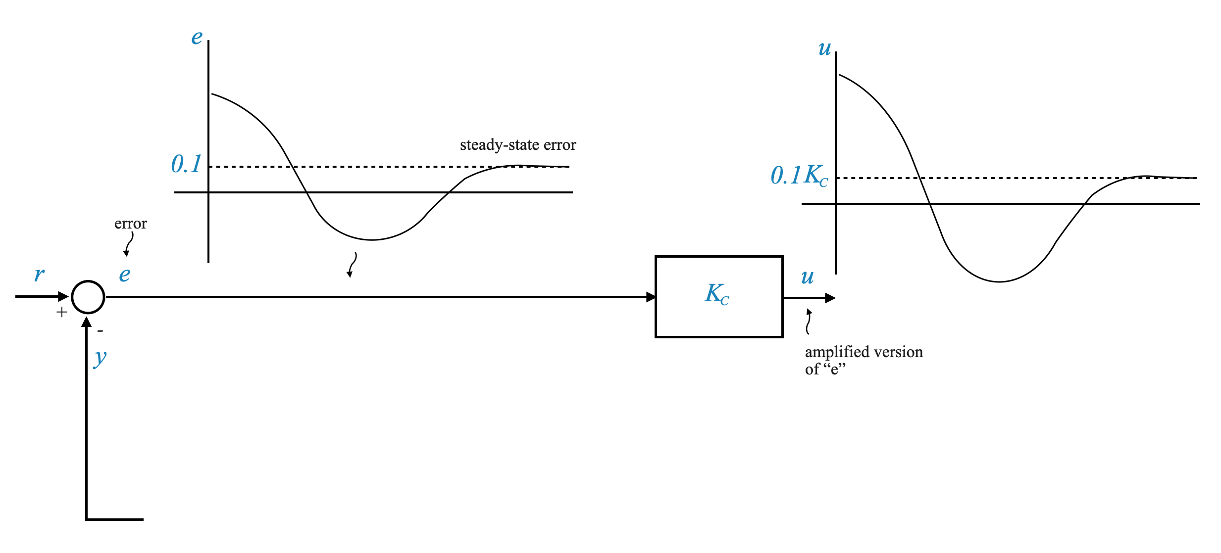
In proportional control, the error provides the energy needed to sustain a new equilibrium. The new equilibrium is obtained using new energy that is only available if the error signal is present. If the error is zero, you go back to the original equilibrium position. However this is not possible because the system is driven to the new situation.

• Role of Integral Control: The integral controller accumulates the error over time, allowing the error to reduce to zero while still providing the necessary control action.

Integral control uses the accumulation of past errors to achieve this, allowing the error to eventually reduce to zero. This is always possible for the type of systems we are considering.

---

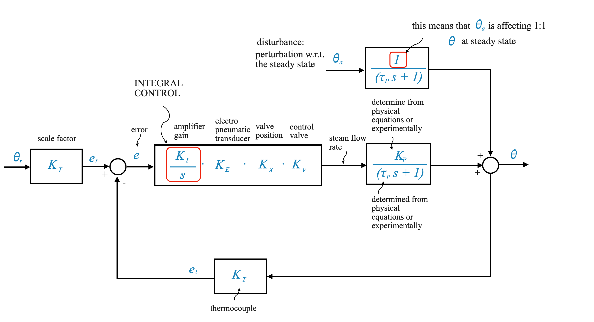
Revisiting the Temperature Control System

We will now revisit the temperature control process discussed previously, focusing on the system’s dynamics, particularly the role of integral control in enhancing system performance.

System Overview

Block Diagram Description

• Reference Temperature: Denoted as \(\theta_r\), the desired temperature setting.
• Sensor and Error Signal: A thermocouple sensor converts \(\theta_r\) into a voltage signal. This voltage is compared with the actual temperature voltage to generate an error signal.
• Amplifier and Transducer: The error signal is amplified (gain \(K_A\)) and then sent to an electropneumatic transducer (constant \(K_e\)).
• Valve Positioner and Gain: The transducer signal controls a valve positioner (constant (K_x)) to regulate flow rate, influenced by valve gain \(K_v\).
• Process Transfer Function: Represented as \(\frac{K_p}{\tau_p s + 1}\).
• Disturbance Effect: Modeled as \(\frac{1}{\tau_p s + 1}\), where \(\theta_a\) is the ambient temperature disturbance.

System Dynamics and Stability

When we assumed that the plant was a first-order system and that the various components can be approximated as zero-order: - Transient Performance: Larger loop gain (\(K\)) improves transient performance by reducing the system’s time constant. - Steady State Error: Larger \(K\) also reduces steady state error. - Constraints on Gain: High gain \(K\) can lead to component saturation and nonlinear behavior, limiting the system’s linear response range. Additionally, the dynamics of the various components cannot be neglected leading to potential instability.

Integral Control in Temperature Systems

Addressing Command Signal Changes

• Scenario: Consider a requirement to increase the chamber temperature by 10 degrees.
• Command Change: This necessitates a change in \(\theta_r\) by the same amount.

Integral Control Mechanism

• Error Signal Dynamics: With integral control, the system can handle changes in command signal while maintaining stability and performance.

Mathematical Expression:

\[ u(t) = K_I \int e(t) \, dt \]

Comments: - Role in System Stability: Integral control enables the system to automatically adjust to new equilibriums without compromising stability.

• System Adaptability: The integral controller adjusts the control action over time based on accumulated error, leading to a zero steady-state error even with command changes.

• System Adaptability: The integral controller adjusts the control action over time based on accumulated error, leading to a zero steady-state error even with command changes.

There will be a price to pay: integral control might lead to instability even more than the usage of a simple proportional controller.

Implementing Integral Control in Temperature Systems

Let’s replace the amplifier \(K_A\) with an integral controller \(K_I/s\).

System Dynamics: The system now includes the integral controller, the Electropneumatic transducer (\(K_e\)), valve positioner (\(K_x\)), and valve gain (\(K_v\)).

Based on this block diagram we can then write the mathematical equations:

\[ (K_t\theta_r - K_t\theta)\cdot \Big(\frac{K_I}{s}K_eK_xK_v \Big) \Big(\frac{K_p}{\tau_ps+1} \Big) + \frac{1}{\tau_ps+1} \theta_a = \theta \]

We can then rearrange the equation to isolate \(\theta(s)\) on one side.:

\[ (\tau_p s + 1)\theta(s) + \frac{K}{s} \theta(s) = \frac{K}{s} \theta_r(s) + \theta_a(s) \]

where \(K = K_tK_IK_eK_xK_vK_p\).

And hence:

\[ \Big(\tau_p s + 1 + \frac{K}{s}\Big) \theta(s) = \frac{K}{s} \theta_r(s) + \theta_a(s) \]

or equivalently:

\[ \Big(\tau_p s^2 + s + K \Big) \theta(s) = K \theta_r(s) + s\theta_a(s) \]

Steady State Performance with Integral Control

We would like now to calculate the steady state for a step input in command and in disturbance

• Command Input Response: For a step input command, the steady-state output \(\theta_{ss}\) is equal to 1, irrespective of \(K\), indicating zero steady-state error.

\[ \frac{\theta(s)}{\theta_r(s)} = \frac{K}{\tau_p s^2 + s + K} \]

Applying \(\theta_r(s)=\frac{1}{s}\), we can calculate \(\theta_{ss}\):

\[ \theta_{ss} = \lim_{s \to 0} s \theta(s) = s \frac{K}{\tau_p s^2 + s + K} \frac{1}{s} = 1\]

This is true for all possible values of \(K\) and the steady state error is zero.

• Disturbance Response: In response to a step disturbance \(\theta_a(s)=\frac{1}{s}\), the steady-state output \(\theta_{ss}\) becomes zero, effectively rejecting the disturbance:

\[ \frac{\theta(s)}{\theta_a(s)} = \frac{s}{\tau_p s^2 + s + K} \]

\[ \theta_{ss}|_{dist} = 0 \]

Transient Performance with Integral Control

Let’s get back to the response to the input:

\[ \frac{\theta(s)}{\theta_r(s)} = \frac{K}{\tau_p s^2 + s + K} \]

Comments:

• The addition of integral control changes the system from first-order to second-order.

Remember that with a proportional controller the system was a first-order system with form \(\frac{\theta(s)}{\theta_r(s)} = \frac{K}{\tau_p s + 1 + K}\)

For this first-order system the pole is:

\[ s= \frac{-(1+K)}{\tau_p} \]

When we increase \(K\) the pole remains on the left-hand plane and moves from \(s=\frac{-1}{\tau_p}\) (when \(K=0\)) to the left and its response gets faster and faster.

For the second-order system, the poles are the roots of:

\[ \tau_p s^2 + s + K = 0 \]

When \(K=0\), the roots are \(s=0\), and \(s=\frac{-1}{\tau_p}\).

Note that if there is a pole at the origin the transiet will never decay.

As we increase the gain \(K\) the two poles will move closer together, until at some point they will become complex conjugate.

Limitations in Improvement

• Limit on Transient Performance: Integral control imposes a limit on the improvement of transient performance, as poles can only be driven to a certain point (see root locus plot below).
• Oscillatory Response: Increasing (K) can lead to oscillatory behavior, a direct consequence of integral control.

import numpy as np
import matplotlib.pyplot as plt
from control import tf, root_locus

# System parameters
tau_p = 1  # For example, let's take tau_p as 1

# Define the characteristic equation of the system with integral control
# The characteristic equation is tau_p * s^2 + s + K = 0

# For the root locus, we consider the open-loop transfer function G(s)H(s)
# G(s)H(s) = K / (tau_p * s^2 + s)
# This is equivalent to a system with a numerator [K] and a denominator [tau_p, 1, 0]

numerator = [1]  # Coefficient for K
denominator = [tau_p, 1, 0]  # Coefficients of s^2, s, and constant term for the denominator

# Create the transfer function for the system
system = tf(numerator, denominator)

# Plot the root locus
fig, ax = plt.subplots()
root_locus_data = root_locus(system, Plot=True, ax=ax)

# Add labels and title for clarity
plt.xlabel('Real Axis')
plt.ylabel('Imaginary Axis')
plt.title('Root Locus with Integral Control')
plt.grid(True)

plt.show()

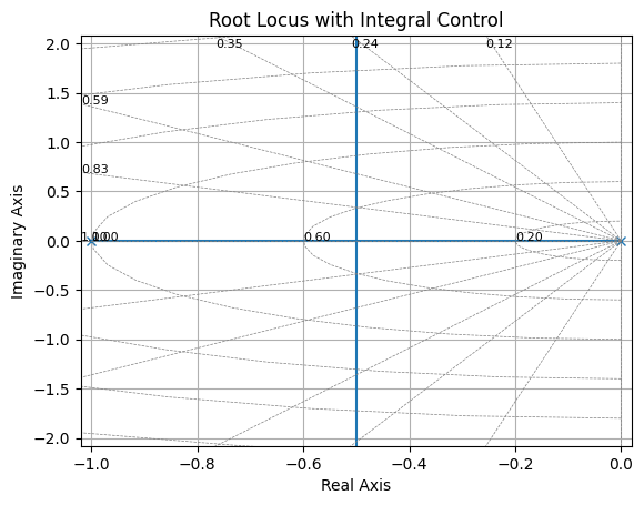
Influence of Poles on System Response

• Poles: In control theory, the poles of a system are the roots of its characteristic equation. They are crucial in determining the system’s behavior over time, particularly its stability and transient response.

• Complex Plane Representation: Poles are represented in the complex plane, where the horizontal axis is the real axis and the vertical axis is the imaginary axis (jω axis).

• Location of Poles: The location of poles in the complex plane significantly impacts how the system responds to inputs.

• Real Axis Proximity: Poles closer to the jω axis (imaginary axis) have a smaller real part. This small real part implies a slower decay rate of the system’s transient response.

• Dominant Poles: Poles that are closer to the jω axis are often referred to as “dominant poles” because they have a more pronounced effect on the system’s transient behavior. Their slower decay rate means that they dictate the overall response of the system, especially in the transient phase.

Design Considerations

• With referect to the root locus above, the dominant pole cannot be moved further left, hence limiting the dynamic response we can obtain.
• When designing control systems, engineers often aim to position the dominant poles in a way that achieves a desired balance between quick response and stability. Poles that are too close to the jω axis may result in slow response times, while poles too far into the left-half plane may cause the system to respond too quickly, potentially leading to overshoot and instability.
• Transient vs. Steady-State Response: The dominant poles primarily affect the transient response of the system. Once the transient effects have decayed, the steady-state behavior is determined by other factors, such as the system’s steady-state gain and the type of controller used (e.g., proportional, integral, derivative).

In this case, the poles do not move to the right (become unstable). However, if one of the time constant of our components start to have an effect that might easily lead the system to instability (the system becomes at least of third order which might have poles going to RHP for high K).

Introduction to Derivative Control

Let’s now consider the following error:

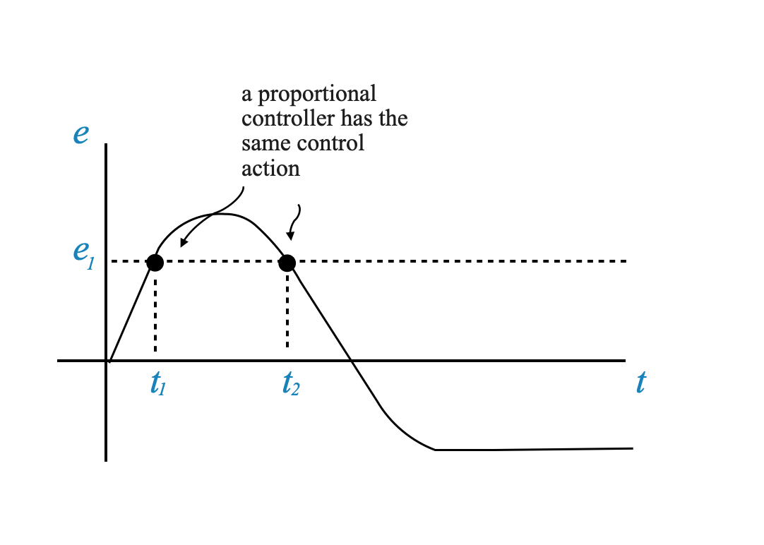
At times $ t_1 $ and $ t_2 $, a proportional controller would exhibit identical control actions since the magnitude of the error is the same at both instances. Nonetheless, the scenarios at $ t_1 $ and $ t_2 $ are distinctly different: at $ t_1 $, the error is increasing, whereas at $ t_2 $, the error is on a decreasing trend.

Intuitively, we would prefer varied control actions in these situations. Specifically, at $ t_1 $, a more aggressive control action might be desirable to prevent the error from escalating. By considering the error’s rate of change, or its slope, we can distinguish between these scenarios. This slope effectively informs the controller about potential future errors, enabling a more predictive and adaptive response.

This is what a derivative control does: it introduces a signal that is not only proportional to the magnitude of the error (proportional control), but on the derivative of that signal.

Derivative Control Concept

Predictive Nature of Derivative Control

• Prediction through Derivative: Derivative control predicts future errors (through the slope of the error signal) and adjusts the control action accordingly, providing more damping during transients.

Equation:

\[ U(s) = K_c (1 + T_D s) E(s) \]

• Effectiveness: Derivative control is effective during transient periods but has no impact on steady-state error.
  • If the steady error becomes constant, i.e., when you reach steady state, the derivative is zero and the effect of derivative control is zero (see error plot above).
  • At steady state the derivati control loses its role and it only proportional and integral control that can support it.

Implementing Derivative Control in Control Systems

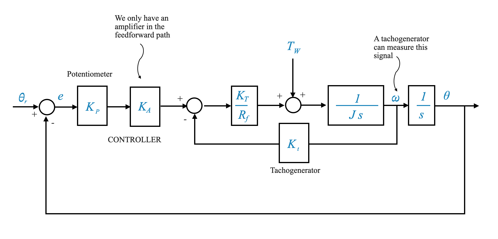
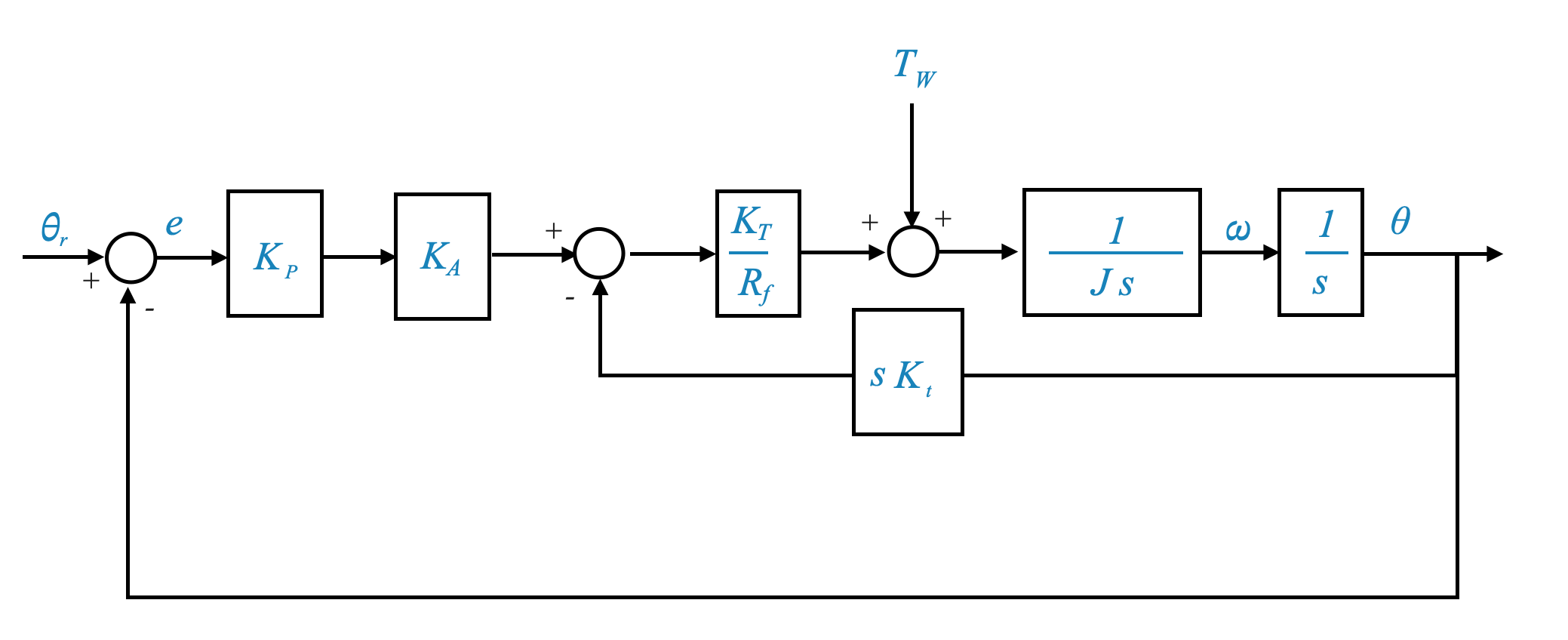
We now shift our focus to the practical aspects of implementing derivative control in control systems. We’ll discuss the challenges and alternatives in employing derivative control, particularly in the context of a position control system.

We have the following control action:

\[ U(s) = K_c (1 + T_D s) E(s) \]

Noise Amplification Issue

• Derivative of High-Frequency Noise: Derivative control can amplify high-frequency noise signals, potentially disrupting the system’s performance.

• Example Scenario: Consider a noise signal \(0.01 \sin(10^3 t)\). The amplitude of this signal is very small, and it is high frequency. In proportional control, most likely we do not need to consider this explicitely because the system itself is a low pass filter.

In derivative control, the derivative of this signal is $10^3 (10^3 t) = 10 (10^3 t) $, which significantly amplifies the noise.

The derivative action $ T_D s $ applied to a noise signal can lead to a large magnitude signal that may overshadow the actual error signal.

For this reason the derivative control described above is only theoretical and never implemented in practise. You always apply a suitable low pass filter for the implementation (we will see this later).

For the purpose of this notebook it is assumed that high frequency noise are not part of the problem or they have been filtered out appropriately.

Alternatives to Standard Derivative Control

Let’s see what alternatives we can have using a position control system. For this we will revisit the Position Control System we analysed in a previous notebook and reported below.

Note that we have made a few simplifications: - Plant is inertial only. - Inductance is neglected.

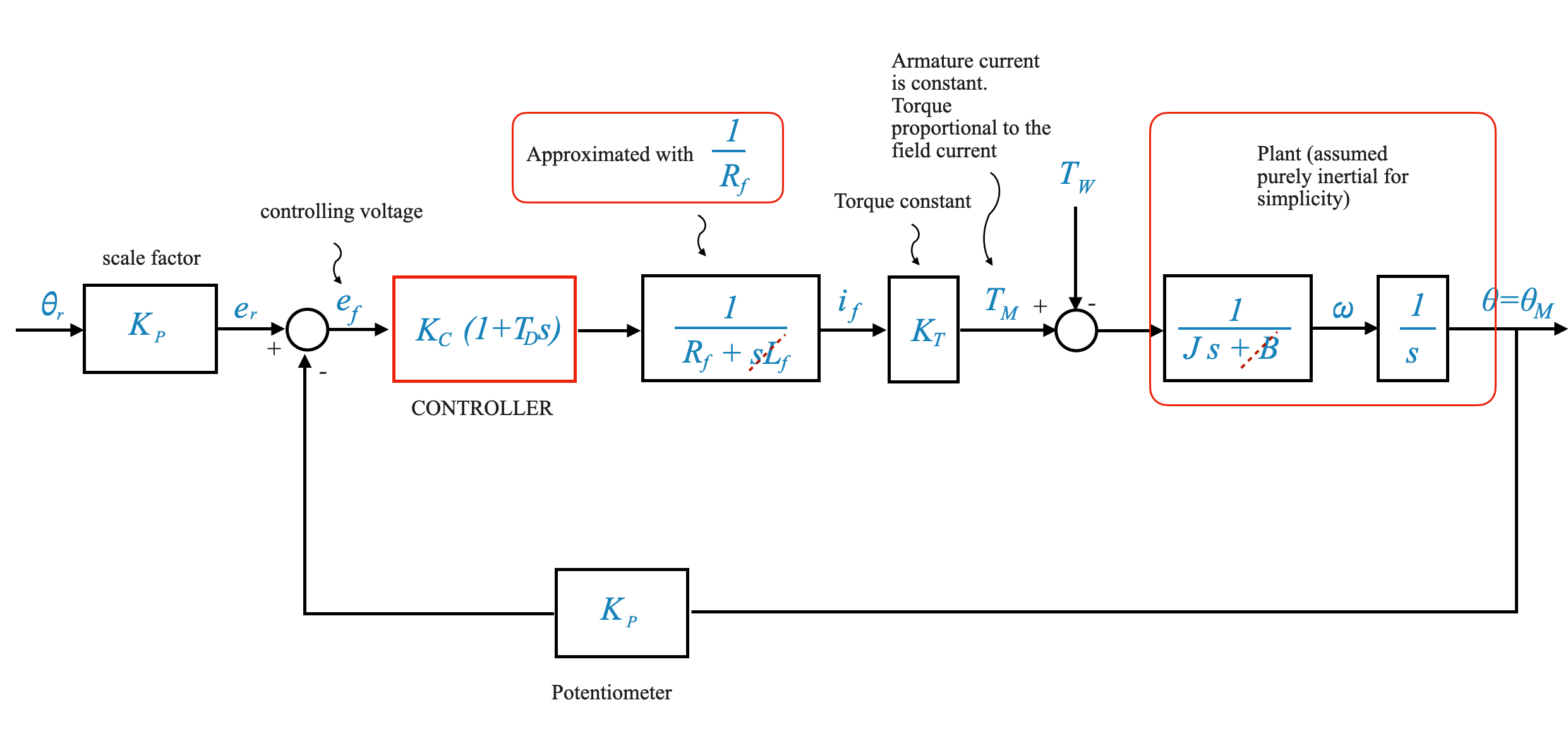
From this we can calculate the equation (note that the sign of the disturbance torque \(T_W\) is not important):

\[ \Big[ \Big(K_p\theta_r - K_p\theta\Big) K_c \Big(1+T_Ds\Big)\frac{K_T}{R_f} + T_W \big] \frac{1}{Js^s} = \theta \]

which can be written as:

\[ Js^s\theta + K_pK_C\frac{K_T}{R_f}\Big(1+T_Ds\Big)\theta = K_pK_C\frac{K_T}{R_f}\Big(1+T_Ds\Big)\theta_r + T_W \]

we can set: \(K = K_pK_C\frac{K_T}{R_f}\) and obtain:

\[ \Big(Js^2 + K T_D s + K\Big)\theta(s) = K(1+T_Ds)\theta_r + T_W \]

and finally we can write the Transfer Function:

\[ \frac{\theta(s)}{\theta_r(s)} = \frac{K (1 + T_D s)}{Js^2 + K T_D s + K} \]

And the “personality parameters” of the systems are:

\[ \omega_n = \sqrt{\frac{K}{J}} \]

\[ 2\zeta\omega_n = \frac{KT_D}{J} \rightarrow \zeta=\frac{T_D}{2}\sqrt{\frac{K}{J}} \]

The effect of the derivative control on the transient is visibile through \(\zeta\). You can increase the damping increasing \(T_D\).

Additional comments:

If we look at the transfer function we notice: - The denominator is a second-order system - The numerator has one zero

When a step change is introduced in the command signal (\(\theta_r\)), such as \(\theta_r = \frac{1}{s}\) in the Laplace domain, and this signal interacts with a derivative control element characterized by \(T_Ds\) (see numerator of the transfer function above), it results in the generation of an impulse, or a spike.

This phenomenon occurs because differentiating a step function, which essentially remains constant after the initial change, produces an impulse:

\[ T_Ds \cdot \frac{1}{s} \rightarrow T_D \cdot \delta(t) \]

This implies that in response to a step change, a derivative controller produces an exceptionally high initial output, commonly referred to as a spike. This behavior can be interpreted as the control system’s immediate effort to counter a sudden and significant change in the error.

However, such a spike in the controller’s output is not always desirable. While it represents an immediate response to the error change, it can be likened to introducing a disturbance into the system only to subsequently correct it. This could potentially lead to issues such as system instability or excessive overshoot, especially in systems sensitive to rapid changes.

Smoothing the controller’s response:

To address this issue, control systems are often equipped with additional filtering mechanisms. Alternatively, a modified approach to derivative control is employed, one that does not react as intensely to high-frequency components of the error signal. These design strategies help in smoothing out the controller’s response, preventing the abrupt spike and ensuring a more stable system behavior.

And the presence of the Tachogenerator is equivalent to:

Rather than computing the derivative of the output signal, one can employ a tachogenerator to generate a feedback signal that is proportionate to the output’s rate of change.

This method circumvents the challenges typically encountered when differentiating the input command, specifically the issues of noise amplification and the creation of spikes when there are sudden changes in the command signal.

In the actual implementation of this system, no derivative operation is conducted. While the model includes a derivative term (\(sK_t\)), this differentiation does not occur in practice.

It’s important to note, however, that this approach is not universally applicable. For instance, in temperature control systems, there isn’t an inherent signal within the system that directly represents the derivative of the variable being controlled.

In motion control, this is possible, in process control this is generally not possible. In this case, we add suitable filters to avoid spikes.

Instead of directly calculating the derivative of the output signal, a tachogenerator can be utilized to produce a feedback signal that correlates with the rate of change of the output. This strategy effectively addresses typical issues associated with direct differentiation of the input command. These issues include the amplification of noise and the generation of spikes, especially when the command signal undergoes abrupt changes.

In practical implementations of such a system, an actual derivative calculation is not performed. The system’s model might include a derivative term represented as $ sK_t $, but in reality, this differentiation process is not carried out. The tachogenerator inherently provides a signal that reflects the derivative, thus bypassing the need for explicit differentiation.

However, it is crucial to recognize that this method is not universally applicable across all types of control systems. For example, in temperature control systems, there typically isn’t a readily available signal that inherently represents the derivative of the temperature. Such systems lack an equivalent to the tachogenerator used in motion control systems, where the derivative feedback is naturally integrated.

In contexts like process control, where directly obtaining a derivative signal is not feasible, alternative strategies must be employed. These often involve adding suitable filters to the control system. These filters are designed to mitigate or eliminate the unwanted effects, such as spikes, that can occur when using derivative control. This approach ensures smoother system performance and reduces the risk of instability or excessive response to high-frequency disturbances.