PID Control

PID Simulation

!pip install slycot
!pip install control

Collecting slycot
Installing collected packages: slycot
Successfully installed slycot-0.2.0
Collecting control
  Using cached control-0.7.0-py2.py3-none-any.whl
Requirement already satisfied: numpy in /Users/jeff/anaconda3/lib/python3.6/site-packages (from control)
Requirement already satisfied: scipy in /Users/jeff/anaconda3/lib/python3.6/site-packages (from control)
Requirement already satisfied: matplotlib in /Users/jeff/anaconda3/lib/python3.6/site-packages (from control)
Requirement already satisfied: six>=1.10 in /Users/jeff/anaconda3/lib/python3.6/site-packages (from matplotlib->control)
Requirement already satisfied: python-dateutil>=2.0 in /Users/jeff/anaconda3/lib/python3.6/site-packages (from matplotlib->control)
Requirement already satisfied: pytz in /Users/jeff/anaconda3/lib/python3.6/site-packages (from matplotlib->control)
Requirement already satisfied: cycler>=0.10 in /Users/jeff/anaconda3/lib/python3.6/site-packages (from matplotlib->control)
Requirement already satisfied: pyparsing!=2.0.4,!=2.1.2,!=2.1.6,>=2.0.1 in /Users/jeff/anaconda3/lib/python3.6/site-packages (from matplotlib->control)
Installing collected packages: control
Successfully installed control-0.7.0

import numpy as np
import matplotlib.pyplot as plt
import control.matlab as control

# control constants
Kc = 0.85
tauI = 10000

# control transfer function
Gc = Kc*control.tf([tauI,1],[tauI,0])

# model transfer functions
Gp = control.tf([0.31],[16,1])*control.tf([1],[135,1])

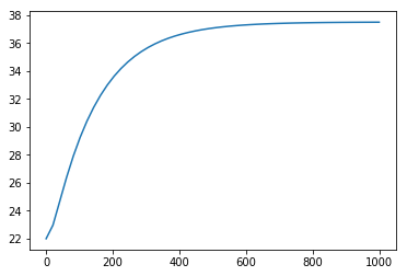
t = np.linspace(0,1000)
y,t = control.step(Gp,t)
plt.plot(t,50*y + 22)

# control constants
Kc = 2
tauI = 60

# control transfer function
Gc = Kc*control.tf([tauI,1],[tauI,0])

t = np.linspace(0,1000)

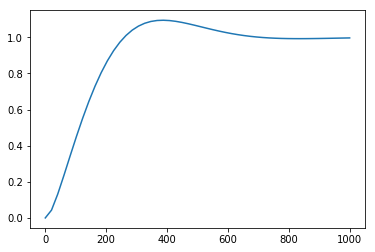
H = Gp*Gc/(1+Gp*Gc)
y,t = control.step(H,t)
plt.plot(t,y)

PID Implementation

Reference Conditions

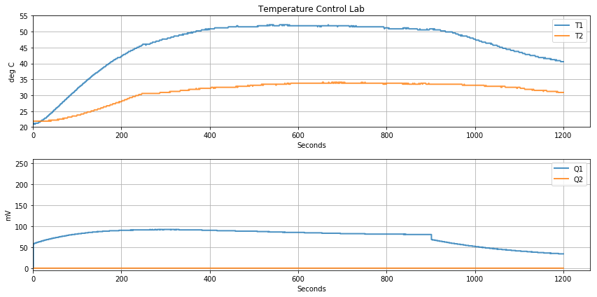
One of the implementation issues for PID control of the Temperature Control Lab is choice of reference conditions. One reason is that the linearization on which PID analysis is based is only valid in some ‘neighborhood’ of a nominal operating condition. But perhaps a more typical situation in most practical

import sys
sys.path.append('..')
from tclab import TCLab, clock, pid

# ambient and reference values
Tamb = 20
Tref = 50
uref = (Tref - Tamb)/0.85

# control parameters
b = 1              # setpoint weighting
kp = 0.8          # proportional control gain
ki = kp/60

# sampling period
tf = 1200           # experiment length (sec.)
h = 1               # sample time (sec.)

# setpoint function
def Tset(t):
    if t <= 900:
        return 50
    else:
        return 35


bi = ki*h

r = Tset(0) - Tref
y = Tamb - Tref

P = kp*(b*r - y)
I = 0

uref,P,I,r

(35.294117647058826, 24.0, 0, 0)

# device initialization
with TCLab() as a:
    a.initplot(tf)
    for t in clock(tf,h):
        r = Tset(t) - Tref
        y = a.T1 - Tref
    
        P = kp*(b*r - y)
        v = P + I
    
        u = max(0,min(200,v + uref))
        I += bi*(r-y)
    
        a.Q1 = u
        a.updateplot()

TCLab disconnected successfully.