Control System Components

Automatic control systems are ubiquitous in various industries and applications. They help maintain desired output conditions by adjusting the input accordingly. One fundamental aspect of understanding these systems is the concept of analogous systems and understanding the components that make up a control system.

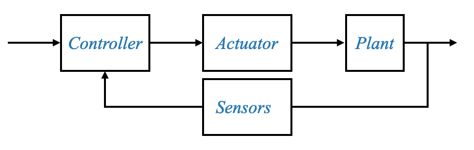
In automatic control systems, the entire process can be visualized as a sequence of interconnected components. This sequence begins with the plant, which is essentially the system we aim to control. The plant is driven by an actuator, and the power to this actuator is controlled by the controller, which is the brain of our system. The controller makes decisions based on feedback it receives from sensors that monitor the system.

Control systems consist of various components that work together to achieve a desired output.

In our discussion, we primarily focus on mechanical systems, but other systems like thermal or liquid-based systems also exist as we saw.

Components of the Control System:

• Plant: The primary system that needs to be controlled. This is often a mechanical system in our discussions, but it can also be a thermal system, a liquid system, or any other system that requires control.
• Actuator: A device that drives or controls the plant. For mechanical systems, motors are common actuators.
• Controller: The brain of the system. It decides how to drive the actuator based on the difference between the desired output and the actual output. This can be an operational amplifier circuit (Op-Amp) or even a digital computer in modern systems.
• Sensor: A device that measures the actual output of the plant. It often needs noise filters to remove high-frequency noise and amplifiers to boost its signals to usable levels.

The brain of the control system, the controller, is often electrical in nature. Today, most controllers are either Op-Amp circuits (legacy) or digital computers. Hydraulic or pneumatic controllers were used in the past. The trend is moving toward these controllers because of their versatility and efficiency.

Your role:

1. Designing noise filters to ensure that high-frequency noise from sensors doesn’t interfere with the system.
2. Amplifying or conditioning sensor outputs to make them compatible with the standard input signals or to suit the controller hardware. For example, sensor output can be millivolt or milliamper, and require amplification to use them together with the levels of the input signal and with the controller.
3. Designing the controller, which is the most critical part of the system.

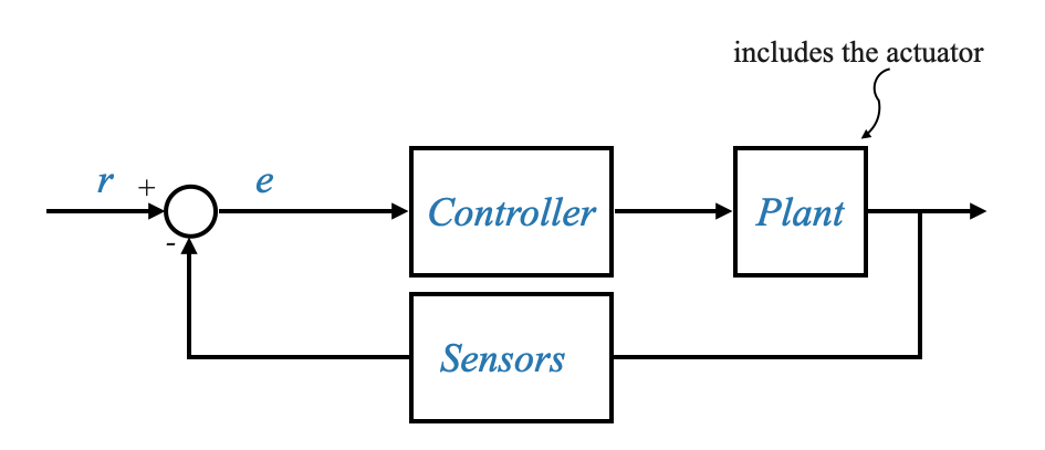
Let’s make the diagram more precise:

The controller can respond to the error signal in various manners. One approach is to amplify the error, referred to as a Proportional controller. Another method involves controllers that produce a signal based on both the error and its integral. This results in a signal composed of two parts: one directly proportional to the error and another proportional to the accumulated error over time. We talk about Proportional and Integral Controllers in this case.

In addition to these, there’s the Proportional-Derivative (PD) controller, which not only responds to the present error but also to the rate of change of this error. By considering the derivative or the rate at which the error is changing, the PD controller can anticipate future errors and act more responsively, making it especially useful in scenarios where swift corrections are essential.

Then there’s the Proportional-Integral-Derivative (PID) controller, which combines all three strategies. It considers the present error (proportional), the accumulation of past errors (integral), and the rate of change of the error (derivative). By using all three components, the PID controller offers a comprehensive approach to error correction, ensuring steady-state accuracy, quick response, and anticipation of future errors. This makes the PID controller one of the most widely used control strategies in various industries due to its adaptability and efficiency in diverse control scenarios.

1. Proportional (P) Controller: \[ u(t) = K_p \cdot e(t) \]

Where: - $ u(t) $ is the control output. - $ K_p $ is the proportional gain. - $ e(t) $ is the error signal.

2. Proportional-Integral (PI) Controller: \[ u(t) = K_p \cdot e(t) + K_i \int e(t) \, dt \]

Where: - $ K_i $ is the integral gain.

The majority of the industrial controllers are PI controllers.

3. Proportional-Derivative (PD) Controller:

\[ u(t) = K_p \cdot e(t) + K_d \frac{d e(t)}{dt} \]

Where: - $ K_d $ is the derivative gain.

4. Proportional-Integral-Derivative (PID) Controller:

\[ u(t) = K_p \cdot e(t) + K_i \int e(t) \, dt + K_d \frac{d e(t)}{dt} \]

In these equations: - $ e(t) $ represents the error signal, which is the difference between the setpoint and the process variable (or the measured output). - The gains $ K_p $, $ K_i $, and $ K_d $ determine the strength of the controller’s response to the error, its accumulation, and its rate of change, respectively. Adjusting these gains allows for tuning the controller’s performance to suit specific applications.

These can be easily implemented as analog controllers using Op-Amps.

Analog Controllers

Operational amplifiers (Op-Amps) are crucial components in control systems. They can act as amplifiers, integrators, or differentiators, depending on their configuration.

1. Proportional Controller (P):

• Circuit:

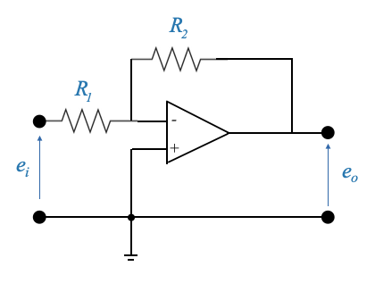
• Transfer function:

\[ \frac{E_0(s)}{E_i(s)}=-\frac{R2}{R1} \]

• Note that with two circuits in serie we can get rid of the minus sign.

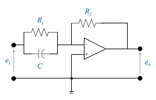
2. Proportional-Integral Controller (PI):

• Circuit:

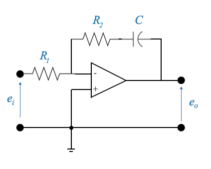
• Transfer function:

\[ \frac{E_0(s)}{E_i(s)}=-\frac{R_2+\frac{1}{sC}}{R_1} = -\frac{R_2}{R_1} - \frac{1}{R_1C}\frac{1}{s} \]

that we can write it as:

\[ e_0(t) = -\frac{R_2}{R_1}e_i(t) - \frac{1}{R_1C}\int_{0}^{t}e_i(\tau)d\tau \]

3. Proportional-Derivative Controller (PD):

• Circuit:

• Transfer function:

\[ \frac{E_0(s)}{E_i(s)}=\frac{\frac{R_2}{R_1\frac{1}{sC}}}{R_1+\frac{1}{sC}} \]

and with simple manipulations we can obtain the standard structure.

4. Proportional-Integral-Derivative Controller (PID):

• Circuit:

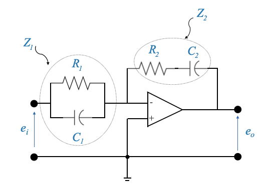
• Transfer function:

\[ \frac{E_0(s)}{E_i(s)} = -\frac{Z_2(s)}{Z_1(s)} \]

where

\[ Z_1 = \frac{R_1}{R_1C_1s+1} \;\;\;\; Z_2=\frac{R_2C_2s+1}{C_2s} \]

---

Op-Amps

• An op-amp, short for operational amplifier, is a type of electronic component that amplifies voltage. It’s essentially a device that takes in two voltage inputs, compares them, and outputs the difference between these voltages multiplied by a very high number. The two inputs are known as the inverting input (marked with a minus sign) and the non-inverting input (marked with a plus sign). The output attempts to make the difference between the inputs zero by amplifying the voltage difference.

• Op-amps are fundamental components in electronics, widely used for signal conditioning, filtering, and to perform mathematical operations such as addition, subtraction, integration, and differentiation, hence the name “operational” amplifier. Their capability to amplify the difference between the voltages at their two inputs (the non-inverting “+” and the inverting “-”) is what makes them so useful across various applications. The actual behavior of an op-amp in a circuit depends on how it is configured, including the external components connected to it, which can control its gain and other characteristics.

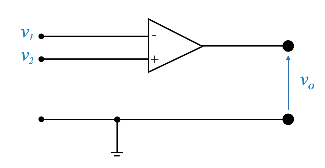
• The input voltages \(v_1, v_2\) can be DC or AC are often measured with respect to ground which acts as a reference.

• The output voltage is: \[ v_0 = K(v_2-v_1) = -K(v_1-v_2) \]

• \(K\) is called (differential) gain and is usually a very large value. It can be as high as \(1e5\) or \(1e6\) for signal frequencies less than \(10Hz\), and decreases for higher frequencies (goes to \(\approx 1\) for frequencies \(> 1MHz\)).

• It is also called differential amplifier because it amplifies the difference between the inputs \(v_1\) and \(v_2\).

• Since its gain is very high it needs a negative feedback to be stabilised. This negative feedback is hence done on the inverted input (negative).

• In an ideal op-amp no current flows through the input terminals (input impedence is \(\infty\)).

• The load has no effect on the output voltage \(v_o\) (output impedence is zero).

Inverting Amplifier (P)

Let’s analyse the proportional controller once again:

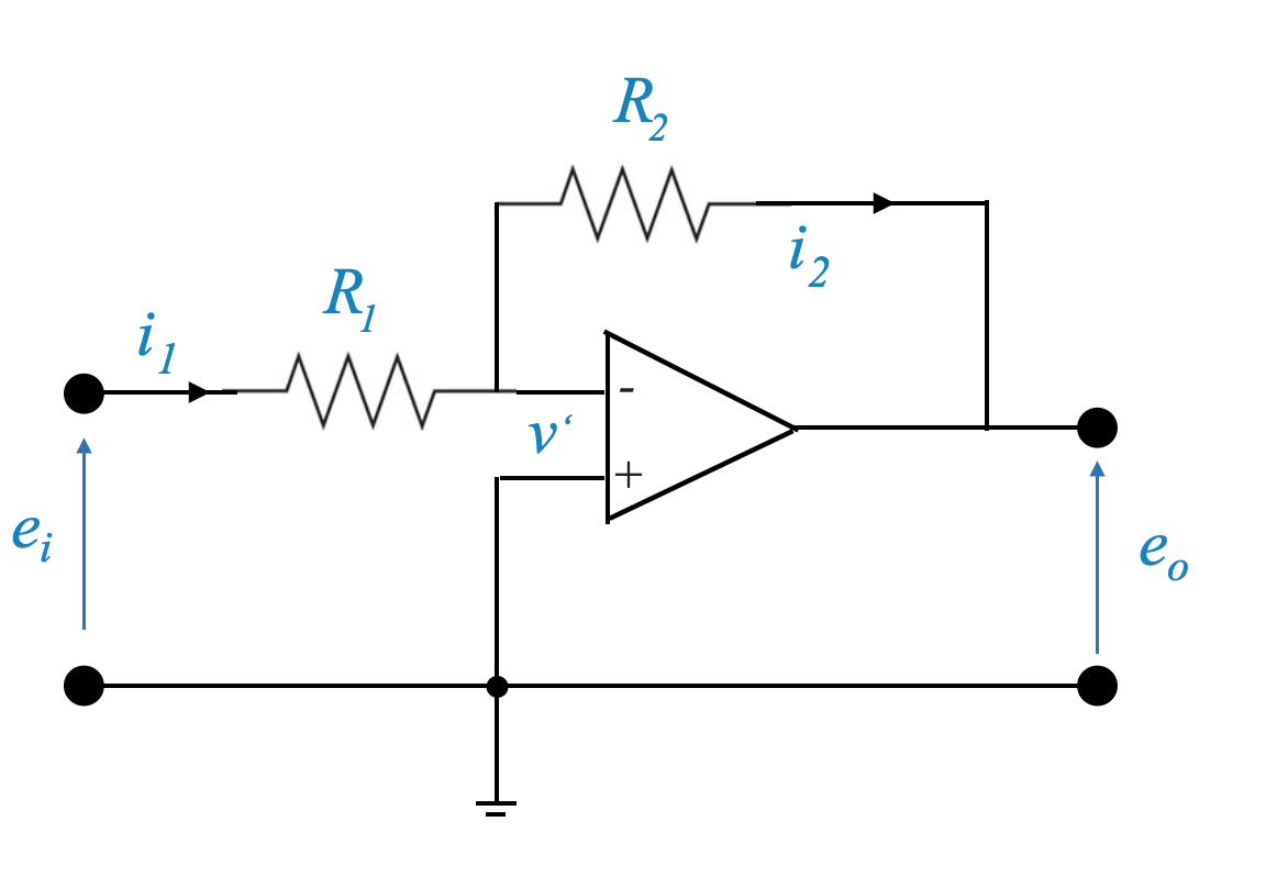
For this circuit we can write:

\[ i_1 = \frac{e_i - v'}{R_1} \]

\[ i_2 = \frac{v' - e_0}{R_2} \]

• Since no current can flow through the op-amp, \(i_1 = i_2\) and hence:

\[ \frac{e_i - v'}{R_1} = \frac{v' - e_0}{R_2} \]

Given that:

\[ v_0 = K(v_2-v_1) = K(0 - v') \]

and \(K >> 1\), \(v'\) must be close to zero: \(v' \approx 0\) and hence:

\[ \frac{e_i}{R_1} = \frac{- e_0}{R_2} \Rightarrow \frac{e_0}{e_i} = \frac{- R_2}{R_1} \]