Fitting Step Test Data to Empirical Models

Read the Data File

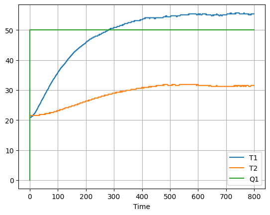
import pandas as pd

df = pd.read_csv('data/step-test-data.csv')
df = df.set_index('Time')
df.plot(grid=True)

Parameter

Fitting the Step Change Data to a First Order Model

For a first-order linear system initially at steady-state, the response to a step input change at \(t=0\) is given by

\[y(t) = y(0) + K(1 - e^{-t/\tau}) \Delta U\]

where \(\Delta U\) is the magnitude of the step change. Converting to notation used for the temperature control lab where \(y(t) = T_1(t)\) and \(\Delta U = \Delta Q_1\)

\[T_1(t) = T_1(0) + K_1(1 - e^{-t/\tau_1}) \Delta Q_1\]

the following cells provide initial estimates for the steady state gain \(K_1\) and time constant \(\tau_1\).

Reading Saved Data

df[['Q1','T1','T2']].plot(grid=True)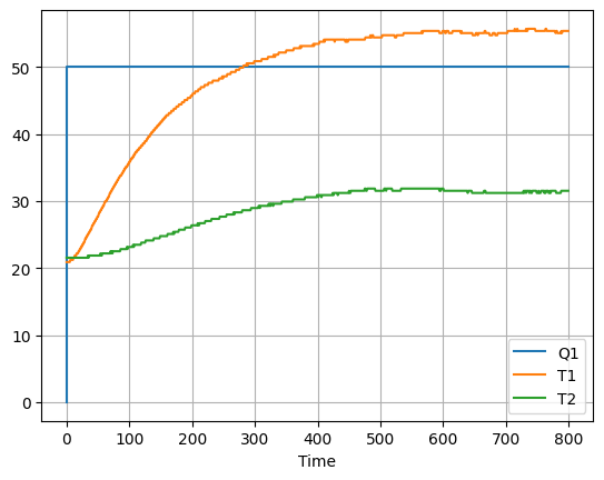

Estimating Gain and Time Constant

In the limit \(t\rightarrow\infty\) the first order model becomes

\[T_1(\infty) = T_1(0) + K_1\Delta Q_1\]

which provides an method for estimating \(K_1\)

\[K_1 = \frac{T_1(\infty) - T_1(0)}{\Delta Q_1}\]

These calculations are performed below where we use the first and last measurements of \(T_1\) as estimates of \(T_1(0)\) and \(T_1(\infty)\), respectively.

T1 = df['T1']
Q1 = df['Q1']

DeltaT1 = max(T1) - min(T1)
DeltaQ1 = Q1.mean()

K1 = DeltaT1/DeltaQ1
print("K1 is approximately", K1)

K1 is approximately 0.6968700000000001

# find when the increase in T1 gets larger than 63.2% of the final increase
i = (T1 - T1.min()) > 0.632*(T1.max()-T1.min())
tau1 = T1.index[i].min()
print("tau1 is approximately", tau1, "seconds")

tau1 is approximately 163.0 seconds

import matplotlib.pyplot as plt
import numpy as np

exp = np.exp
t = df.index

T1_est = T1.min() + K1*(1 - exp(-t/tau1))*DeltaQ1

plt.figure(figsize=(10,5))
ax = plt.subplot(2,1,1)
df['T1'].plot(ax = ax, grid=True)
plt.plot(t,T1_est)
plt.title('Step Test Data Compared to Model')

plt.subplot(2,1,2)
plt.plot(t,T1_est-T1)
plt.grid()
plt.title('Residual Error')

Text(0.5, 1.0, 'Residual Error')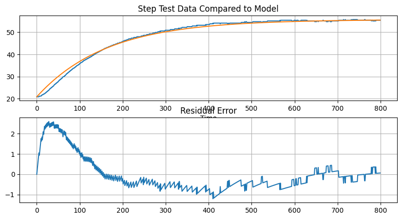

A first order model captures certain features, and provides a reasonably good result as the system approaches a new steady-state. The problem, however, is that for control we need a good model during initial transient. This is where the first-order model breaks down and predicts a qualitatively different response from what we observe.

First Order plus Dead Time

\[T_1(t) = T_1(0) + K (1-e^\frac{t-\theta}{\tau}) Q_{step}\]

import matplotlib.pyplot as plt
import numpy as np
import pandas as pd
from ipywidgets import interact

df = pd.read_csv('data/step-test-data.csv')
df = df.set_index('Time')

T1 = df['T1']
Q1 = df['Q1']
t = df.index

DeltaT1 = max(T1) - min(T1)
DeltaQ1 = Q1.mean()

K1 = DeltaT1/DeltaQ1
i = (T1 - T1.min()) > 0.632*(T1.max()-T1.min())
tau1 = T1.index[i].min()

def fopdt(K=K1, tau=tau1, theta=0, T10=T1.min()):
    def Q1(t):
        return 0 if t < 0 else DeltaQ1
    Q1vec = np.vectorize(Q1)
    T1_fopdt = T10 + K*(1-np.exp(-(t-theta)/tau))*Q1vec(t-theta)
    plt.figure(figsize=(10,5))
    plt.subplot(2,1,1)
    plt.plot(t,T1_fopdt)
    plt.plot(t,df['T1'])
    plt.subplot(2,1,2)
    plt.plot(t,T1_fopdt - T1)
    plt.show()
    
interact(fopdt,K=(0,1,.001),tau=(50,200,.5),theta=(0,50,.5),T10=(15,25,.1))

<function __main__.fopdt(K=0.6968700000000001, tau=163.0, theta=0, T10=20.9)>

Second Order

SEMD Eqn. 5-48

\[T_1(t) = T_1(0) + K\left(1 - \frac{\tau_1 e^{-t/\tau_1} - \tau_2 e^{-t/\tau_2}}{\tau_1 - \tau_2}\right)Q_1(t)\]

import matplotlib.pyplot as plt
import numpy as np
import pandas as pd
from ipywidgets import interact

df = pd.read_csv('data/step-test-data.csv')
df = df.set_index('Time')

T1 = df['T1']
Q1 = df['Q1']
t = df.index

DeltaT1 = max(T1) - min(T1)
DeltaQ1 = Q1.mean()

K1 = DeltaT1/DeltaQ1
i = (T1 - T1.min()) > 0.632*(T1.max()-T1.min())
tau1 = T1.index[i].min()

def secondorder(K=K1, tau1=tau1, tau2=40, T10=T1.min()):
    def Qscalar(t):
        return 0 if t < 0 else DeltaQ1
    Q = np.vectorize(Qscalar)
    exp = np.exp
    T = T10 + K*(1 - (tau1*exp(-t/tau1) - tau2*exp(-t/tau2))/(tau1-tau2))*Q(t)
    plt.subplot(2,1,1)
    plt.plot(t,T)
    plt.plot(t,df['T1'])
    plt.subplot(2,1,2)
    plt.plot(t,T1 - T)
    plt.show()
    
interact(secondorder,K=(0,1,.001),tau1=(1,200,.1),tau2=(0,200,.1),T10=(15,25,.1))

<function __main__.secondorder(K=0.6968700000000001, tau1=163.0, tau2=40, T10=20.9)>

from scipy.optimize import least_squares
import numpy as np
Qmax = 50

def f(x):
    K,tau1,tau2,T10 = x
    t = df.index
    exp = np.exp
    Tpred = T10 + K*(1 - (tau1*exp(-t/tau1) - tau2*exp(-t/tau2))/(tau1-tau2))*Qmax
    resid = df['T1'] - Tpred
    return resid

ic = [0.86,40,130,20]

r = least_squares(f,ic,bounds=(0,np.inf))
r.x

array([  0.69537389,  19.68872647, 141.40950924,  20.91093839])

And the resulting transfer function is:

\[ G_1(s) = \frac{0.70}{(20s + 1)(141s + 1)} \]