It is key to be able to describe the system in an efficient and useful manner.
- To do this, we describe the system mathematically writing the equations of motion in the form of differential equations.
- We have seen how to model the simplified case of a car driving uphill.
The two most popular representations:
- state space representation
- transfer functions.
Loosely speaking, transfer functions are a Laplace domain representation of your system and they are commonly associated with the era of control techniques labeled classical control theory.
State space is a time domain representation, packaged in matrix form, and they are commonly associated with the era labeled modern control theory.
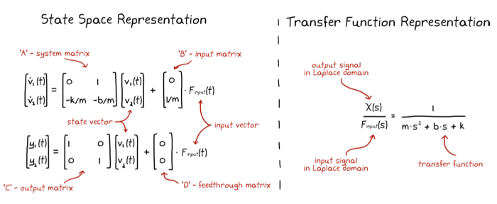 |
- Each representation has its own set of benefits and drawbacks and as a control engineer we need to use what is best for our problem.
- We will focus on Transfer Functions.
- The Laplace Transform takes the Fourier Transform one step forward
- Decomposes a time domain signal into both cosines and exponential functions
- For the Laplace transform we need a symbol that represents more than just frequency, $\omega$
- Need to also account for the exponential aspect of the signal.
- This is where the variable $s$ comes in.
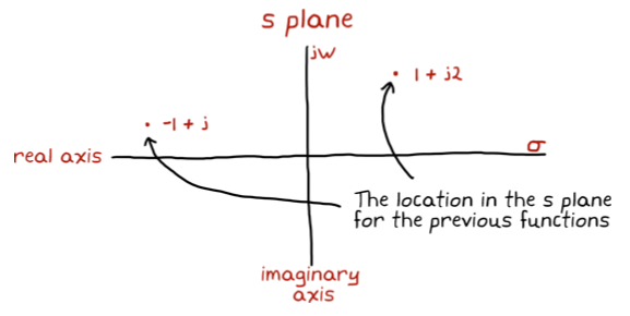
$s$ is a complex number, which means that it contains values for two dimensions:
- one dimension that describes the frequency of a cosine wave
- the second dimension that describes the exponential term.
It is defined as $s = \sigma + j\omega$.
Exponential functions that have imaginary exponents, such as $e^{j2t}$, produce two-dimensional sinusoids through Euler’s formula:
$$e^{j\omega t} = cos(\omega t) + jsin(\omega t)$$
For exponential functions that have real numbers for exponents:
- Negative real numbers give us exponentially decaying signals
- Positive real numbers give us exponentially growing signals.
Two examples are $e^{2t}$, which grows exponentially for all positive time, and $e^{−5t}$, which decays exponentially for all positive time.
fig = plt.figure()

t = np.linspace(-0.2, 1, 20)
plt.plot(t, np.exp(2*t), linewidth=6)
plt.plot(t, np.exp(-5*t), linewidth=6)
plt.grid()
plt.xlabel('time (s)')

Now let’s think about our new variable $s$ which has both a real and imaginary component.
- The equation $e^{st}$ is really just an exponential function multiplied by a sinusoid
$$e^{st} = e^{(\sigma+j\omega)t} = e^{\sigma t}e^{j\omega t}$$
import cmath
fig, axs = plt.subplots(1,3, figsize=(20,5))

t = np.linspace(-0.2, 10, 50) # time range

# s = 1 + j2
s = complex(1, 2)

axs[0].plot(t[:10], np.exp(t[:10]), linewidth=6); axs[0].set_title('exp(t)')
axs[1].plot(t, np.exp(complex(0,2)*t), linewidth=6); axs[1].set_title('exp(j2t)')
axs[2].plot(t, np.exp(t)*np.exp(complex(0,2)*t), linewidth=6); axs[2].set_title('exp(st)')

plt.grid()
plt.xlabel('time (s)')
fig.tight_layout()

fig, axs = plt.subplots(1,3, figsize=(20,5))

t = np.linspace(-5, 5, 50)

# s = -2 + j
s = complex(-2, 1)

axs[0].plot(t[:10], np.exp(-2*t[:10]), linewidth=6); axs[0].set_title('exp(-2t)')
axs[1].plot(t, np.exp(complex(0, 1)*t), linewidth=6); axs[1].set_title('exp(jt)')
axs[2].plot(t, np.exp(-2*t)*np.exp(complex(0, 1)*t), linewidth=6); axs[2].set_title('exp(st)')

plt.grid()
plt.xlabel('time (s)')
fig.tight_layout()

We can combine the two parts of $s = \sigma + j\omega$ into a two-dimensional plane where the real axis is the exponential line and the imaginary axis is the frequency line.
The value of $s$ provides a location in this plane and describes the resulting signal, $e^{st}$, as function of the selected $\omega$ and $\sigma$.
 |
The Laplace transform is an integral transform that converts a function of a real variable $t$ (e.g., $time$) to a function of a complex variable $s = \sigma + j\omega \in \mathbb{C}$ (complex frequency).
$${\displaystyle F(s)={\mathcal {L}}\{f\}(s)=\int _{0}^{\infty }f(t)e^{-st}\,dt.}$$
The inverse Laplace transform is:
$${\displaystyle f(t)={\mathcal {L}}^{-1}\{F(s)\}(t)={\frac {1}{2\pi j}}\lim _{\omega\to \infty }\int _{\sigma -j\omega}^{\sigma +j\omega}e^{st}F(s)\,ds}$$
The Laplace transform is particularly important because it is a tool for solving differential equations: it transforms linear differential equations into algebraic equations, and convolution into multiplication!
- Derivatives and integrals become algebric operations
From a system perspective, the Transfer function expresses the relation between the Laplace Transform of the input and that of the output:
$$ Y(s)=\mathbf{c}^T(s\mathbf{I}-\mathbf{A})^{-1} \mathbf{b} U(s) $$
Properties of the Laplace Transform: relationships between time and frequency
The Laplace transform has a number of properties. These are really useful to calculate the transforms without using its integral definition.
| Property | Time domain | Frequency domain (s) |
|---|---|---|
| Linearity | $af(t)$ + $bg(t)$ | $aF(s)+bG(s)$ |
| Time shift (delay) | $f(t-\tau)$ | $e^{-\tau s}F(s)$ |
| Frequency shift | $f(t)e^{\alpha t}$ | $F(s-\alpha)$ |
| Derivative | $\frac{df}{dt}(t)$ | $sF(s)$ |
| Second Derivative | $\frac{df^2}{d^2t}(t)$ | $s^2F(s) - f(0^-)$ |
| Integral | $\int _{0}^{t}f(\tau )\,d\tau$ = $(u*f)(t)$ | $\frac{1}{s}F(s)$ |
| Convolution | $(f*g)(t)$ = $\int _{0}^{t} f(\tau )g(t$-$\tau )d\tau$ | $F(s)G(s)$ |
| $t\rightarrow\inf$ | $s\rightarrow 0$ | |
| $t\rightarrow 0$ | $s\rightarrow \inf$ |
From this table it is easier to calculate Laplace transforms of known functions:
fig, axs = plt.subplots(1,4, figsize=(10, 5))

t = np.linspace(-10,10,1000)

axs[0].plot(t, delta(t), linewidth=3)
axs[1].plot(t, step(t), linewidth=3)
axs[2].plot(t, ramp(t), linewidth=3)
axs[3].plot(t, ramp(t)**2, linewidth=3)

fig.tight_layout()

If we then want to calculate the Laplace transform of the delta $\delta(t)$ function:
$${\displaystyle F(s)={\mathcal {L}}\{f\}(s)=\int _{0}^{\infty }\delta(t)e^{-st}\,dt.}$$
where
$$\delta(t)=0, \forall t \neq 0 $$ $$\int _{-\infty}^{\infty } \delta(t)dt=1$$
$${\displaystyle F(s)={\mathcal {L}}\{f\}(s)=\int _{0}^{\infty }\delta(t)e^{-st}\,dt.}=e^{-s0}=1$$
Or of the step $1(t)$ function:
$${\displaystyle F(s)={\mathcal {L}}\{f\}(s)=\int _{0}^{\infty }1(t)e^{-st}\,dt.}$$
where
$$1(t)=0, \forall t < 0 $$ $$1(t)=1, \forall t \geq 0 $$
$${\displaystyle F(s)={\mathcal {L}}\{f\}(s)=\int _{0}^{\infty }1(t)e^{-st}\,dt.} = \int _{0}^{\infty}e^{-st}\,dt. = -\frac{e^{-st}}{s} \Bigg|^\infty_0 = -\frac{1}{s} \bigg( \lim_{t\rightarrow \infty} e^{-st} - \lim_{t\rightarrow 0} e^{-st} \bigg) = \frac{1}{s}$$
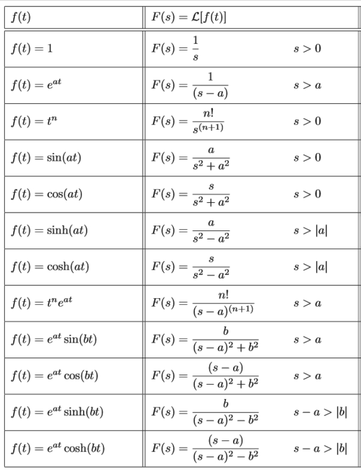
A great thing about working with linear systems is that usually we don’t have to perform the Laplace transform integration by hand.
Most the Laplace transforms for most functions that we will encounter have been solved many times and are available already collected into tables.
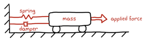
We can model this cart as:
$$m\ddot{x} = F_{input}(t) - F_{dumper}(t) - F_{spring}(t)$$
And since: $F_{spring}(t)=kx(t)$, $F_{dumper}(t)=b\dot{x}(t)$
We obtain:
$$m\ddot{x} + kx(t) + b\dot{x}(t) - F_{input}(t) = 0$$
We can convert this system model into a transfer function:
- it’s a linear,
- time-invariant system,
- there is a single input, $F_{input}$,
- and a single output, $x$.
To calculate the Transfer Function we need to take the Laplace Transform of the impulse response of the system.
To do so, let's set our input to $F_{input}(t)=\delta(t)$ and solve for the response $x(t)$.
$$m\ddot{x} + kx(t) + b\dot{x}(t) - \delta(t) = 0$$
- Solving linear, ordinary differential equations in the time domain can be time consuming.
- We can make the task easier by taking the Laplace transform of the entire differential equation, one term at a time, and solve for the impulse response in the $s$ domain directly.
- Simply take each term and replace with the corresponding $s$ domain equivalent.
| time domain | $\large m\ddot{x} + kx(t) + b\dot{x}(t) - \delta(t) = 0$ |
| $s$ domain | $\large (ms^2 + bs + k)X(s) - 1 = 0 $ |
| $X(s)$ is the impulse response in the $s$ domain | $\large X(s) = \frac{1}{m*s^2 + bs + k}$ |
note that the initial conditions are zeros
To go back to the time domain we could preform the inverse Laplace transform on $X(s)$.
Given:
$$Y(s) = G(s)U(s) = \frac{N(s)}{D(s)}U(s)$$
We want to expand $G(s)$ into the sum of functions for which we already know the inverse transform, then thanks to the linearity we can simply sum them all up to obtain the inverse of the entire function:
Let's suppose we have all distinct poles:
$$ D(s) = \prod^{n}_{k=1}{(s-p_k)}$$
we want to find the coefficient $P_k$ such that:
$$ \frac{N(s)}{\prod^{n}_{k=1}{(s-p_k)}} = \sum^{n}_{k=1}\frac{P_k}{s-p_k}$$
Multiplying for $(s-p_i)$:
$$ (s-p_i)\frac{N(s)}{\prod^{n}_{k=1}{(s-p_k)}} = (s-p_i)\sum^{n}_{k=1}\frac{P_k}{s-p_k}$$
we can obtain:
$$P_i = [(s-p_i)G(s)] \big|_{s=p_i}$$
and finally:
$$ g(t) = \mathcal {L}^{-1}[G(s)]=\mathcal {L}^{-1} \bigg[\sum^{n}_{k=1}\frac{P_k}{s-p_k}\bigg] = \sum^{n}_{k=1} P_k e^{p_kt}$$
If we have muliple poles the decomposition is similar.
For example:
$$G(s) = \frac{s-10}{(s+2)(s+5)}$$
$$P_1=(s+2)\frac{s-10}{(s+2)(s+5)}\bigg|_{s=-2}=-\frac{12}{3}=-4$$ $$P_2=(s+5)\frac{s-10}{(s+2)(s+5)}\bigg|_{s=-5}=\frac{-15}{-3}=5$$
which means that:
$$G(s) = \frac{-4}{(s+2)} + \frac{5}{(s+5)}$$
and finally:
$$ g(t) = \mathcal {L}^{-1}[G(s)] = -4e^{-2t} + 5e^{-5t}$$
Some more on the Laplace transform
- Convert dfferential problems into algebric ones (finding the poles of the system)
- Makes it possible to understand the system output for a given input
- Using the transfer function it is possible to represent the input/output relationship
- Interconnected systems can be represented using block diagrams
- However, it does not allow analysing the controllability and observability of each single block!
The sympy Python module makes it easier to work with Laplace transforms. Let's import it:
import sympy
sympy.init_printing()

# Let's also ignore some warnings here due to sympy using an old matplotlib function to render Latex equations.
import warnings
warnings.filterwarnings('ignore')
And let’s define the symbols with need to work with.
t, s = sympy.symbols('t, s')
a = sympy.symbols('a', real=True, positive=True)
Sympy provides a function called laplace_transform to easily calculate Laplace transforms:
For example, if we want to know the Laplace transform of $e^{\alpha t}$
f = sympy.exp(a*t)
f
F = sympy.laplace_transform(f, t, s, noconds=True)
F
We can define a function to make it easier:
def L(f):
    return sympy.laplace_transform(f, t, s, noconds=True)

def invL(F):
    return sympy.inverse_laplace_transform(F, s, t)
L(f)
invL(L(f))
where $\theta(t)$ is the name used by Sympy for the unit step function.
More transforms:
omega = sympy.Symbol('omega', real=True)
exp = sympy.exp
sin = sympy.sin
cos = sympy.cos
functions = [1,
         t,
         t**2,
         exp(-a*t),
         t*exp(-a*t),
         t**2*exp(-a*t),
         sin(omega*t),
         cos(omega*t),
         1 - exp(-a*t),
         exp(-a*t)*sin(omega*t),
         exp(-a*t)*cos(omega*t),
         ]
functions
Fs = [L(f) for f in functions]
Fs
- We start from the state equations and use the derivate operator of $s$
- We also consider only the forced output of the system
$$\dot{x} = Ax + Bu;\; y = Cx$$
$$sX = AX + BU;\; Y = CX$$
$$(sI-A)X=BU;\; Y = CX$$
$$X = (sI-A)^{-1}BU;$$ $$Y = C(sI-A)^{-1}BU$$
Matrix $G(s)=C(sI-A)^{-1}B$ is the Transfer Function Matrix(or Transfer Matrix).
Each element of $G(s)$ expresses the dynamic relation (there is $s$) between an input channel and an output channel.
$$ \begin{equation} G(s)= \begin{bmatrix} g_{11}(s) & ... & g_{1m}(s)\\ ... & ... & ... \\ g_{p1}(s) & ... & g_{pm}(s) \end{bmatrix} \end{equation} $$$g_{ij}(s)$: Transfer function between $u_j$ and $y_i$, each $g_{ij}(s)=\frac{N(s)}{D(s)}$
$$G(s) = C(sI-A)^{-1}BU$$
- we need to calculate the inverse of a matrix:
$$A^{-1} = \frac{Adjugate(A)}{det(A)}$$
$$\Downarrow$$
$$G(s) = \frac{CAdjugate(sI-A)B}{det(sI-A)}$$
- Roots of the denominator of $G(s)$ (values of $s$ that make $den(G)=0$) are called poles of the system.
- A pole is a value of $s$ that causes $H(s)\rightarrow \inf$ (e.g. $\frac{1}{s}$, when $s=0$, $H(s)\rightarrow \inf$)
- A zero is a value of $s$ that causes $H(s)\rightarrow 0$ (e.g. $s$, when $s=0$, $H(s)=0)$
The poles of the system $G(s)$ are, in general, a subset of the roots of the eq. $det(sI-A)=0$
which are the same as the roots of the characteristic equation: $det(A-\lambda I)=0$
this means that the poles of the system are a subset of the eigenvalue of the matrix $A$.
Stability is the property of the system to stay close to its equilibrium $\bar{x}$ when perturbed $$ \forall ||x_0 - \bar{x} || \le \delta \rightarrow ||x(t) - \bar{x}||\le\epsilon,\;\; \forall t\ge 0$$
Asymptotic stability: the property of the system to go back to its equilibrium when perturbed: $||x(t)|| \rightarrow \bar{x}$, for $t\rightarrow \inf$.
BIBO stability
- A system is BIBO stable (Bounded Input, Bounded Output) if for each limited input, there is a limited output
- For linear systems: BIBO stability if and only if poles of the transfer functions have Re $<0$
Intuition: You can think of stability as meaning that your system’s response decays over time - instability implies the opposite is true, that a finite input will cause your system to respond with increasing amplitude over time, leading to an unstable system.
Note that it is possible to be maginally stable: the system has an infinite, oscillatory response (e.g., sinusoid at constant frequency and amplitude).
Stability margins:
- Even if your system is stable, unmodelled dynamics or parameter variations could make it unstable.
- Stability margins make it possible to evaluate the robustness of the system to these variations.
Note that too much stability is not necessarily a good thing: a system that is too stable means that will tend not to move from its equilibrium even when you desired it to do so.
System stability depends on the eigenvalues of the system matrix $A$ or on the poles of the transfer function:
- eigenvalues with $Re < 0$, system is asymptotically stable
- eigenvalues with $Re \le 0$, and $Re=0$ have multiplicity 1 then the system is stable
When we analyse the stability of linearised systems things can be more complicated.
If the linear system is aymptotically stable, then the non-linear system is stable (around the equilibrium): we can always move close enough to the equilibrium to be inside its region of stability)
If the linear system is marginally stable, we cannot say anything on the non-linear system (other non-linear dynamics become key)
- The stability of a linear system may be determined directly from its transfer function.
- An nth order linear system is asymptotically stable only if all of the components in the response from a finite set of initial conditions decay to zero as time increases, or: $$ \lim \limits_{t\rightarrow\inf} \sum_{i=1}^{n} C_ie^{p_it} $$
where the $p_i$ are the system poles.
For linear systems modelled through their transfer function $G(s)=\frac{N(s)}{D(s)}$, we need to analyse the roots of the characteristic equation $D(s)=0$:
- the system is stable if all the roots of the characteristic equation have negative real part
- the system is stable if all its poles have negative real part.
In order for a linear system to be stable, all of its poles must have negative real parts, that is they must all lie within the left-half of the s-plane. An "unstable" pole, lying in the right half of the s-plane, generates a component in the system homogeneous response that increases without bound from any finite initial conditions. A system having one or more poles lying on the imaginary axis of the s-plane has non-decaying oscillatory components in its homogeneous response, and is defined to be marginally stable.
More structural properties
Stability only depends on the structure of the system (matrix A)
Other aspects:
- What input do we need to take the system into a given state?
- Given the output of a system, how can we determine the state?
Controllability
- A state $x$ is controllable if exists an input $u$ that can take the trajectory of the system from state $0$ to $x$ in finite time.
- A system is controllable if all its states are controllable
Observability
- An initial state is observable if it is possible to determine $x$ measuring the system output $y$
- A system is observable if all its states are observable
$$F(s)=\frac{10}{s^2+12s+40}$$
poles: $-6 \pm \sqrt{36-40} = -6 \pm \sqrt{-4} = -6 \pm j2$
let's call $\alpha_1=-6 + j2$, $\alpha^*_1=-6 - j2$
We can then re-write: $$ F(s) = \frac{10}{[s - (-6+j2)][s - (-6-j2)]} = \frac{10}{(s-\alpha_1)(s-\alpha^*_1)} $$
To calculate the inverse transform we need to find the coefficients:
$$ F(s) = \frac{10}{(s-\alpha_1)(s-\alpha^*_1)} = \frac{A}{s-\alpha_1} + \frac{B}{s-\alpha^*_1} $$where $A$ and $B$ must be complex conjugated: $B=A^*$ (or we would not get real cofficient in $F(s)$).
$$ F(s) = \frac{10}{(s-\alpha_1)(s-\alpha^*_1)} = \frac{A}{s-\alpha_1} + \frac{A^*}{s-\alpha^*_1} $$$$ A = \lim \limits_{s\rightarrow \alpha_1} \frac{10}{(s-\alpha_1)(s-\alpha^*_1)} (s-\alpha_1) = \frac{10}{\alpha_1-\alpha_1^*} = \frac{10}{2j \text{Img(}\alpha_1)} $$this is because $a + jb - (a - jb) = 2jb$
$$ B = \lim \limits_{s\rightarrow \alpha^*_1} \frac{10}{(s-\alpha_1)(s-\alpha^*_1)} (s-\alpha^*_1) = \frac{10}{\alpha^*_1-\alpha_1} = -\frac{10}{2j \text{Img(}\alpha_1)} $$Let's see now the inverse transform:
$$ F(s) = \frac{A}{s-\alpha_1} + \frac{A^*}{s-\alpha^*_1} \rightarrow \mathcal{L^{-1}} \rightarrow Ae^{\alpha_1t} + A^*e^{\alpha^*_1t} $$where we could explicit $\alpha_1 = \sigma + j\omega$, and $A=|A|e^{j\Phi_A}$, $A^*=|A|e^{-j\Phi_A}$
$$ f(t) = Ae^{\alpha_1t} + A^*e^{\alpha^*_1t} = |A|e^{j\Phi_A}e^{(\sigma +j\omega)t} + |A|e^{-j\Phi_A}e^{(\sigma -j\omega)t} = |A|e^{j\Phi_A}e^{\sigma t} e^{+j\omega t} + |A|e^{-j\Phi_A}e^{\sigma t}e^{-j\omega t} $$we can group things together:
$$ f(t) = |A|e^{j\Phi_A}e^{\sigma t} e^{+j\omega t} + |A|e^{-j\Phi_A}e^{\sigma t}e^{-j\omega t} = |A|e^{\sigma t} \big [ e^{j\Phi_A}e^{j\omega t} + e^{-j\Phi_A}e^{-j\omega t} \big ] = |A|e^{\sigma t} \big [ e^{j(\Phi_A+\omega t)} + e^{-j(\Phi_A+\omega t)} \big ] $$and since $\frac{e^{jx}+e^{-jx}}{2}=cos(x)$, we can write the abov expression as:
$$ f(t) = |A|e^{\sigma t} \big [ e^{j(\Phi_A+\omega t)} + e^{-j(\Phi_A+\omega t)} \big ] = 2|A|e^{\sigma t}\cos(\Phi_A+\omega t) $$As expected we have an oscillatory term that could decrease or increase depending on the value of $\sigma$ (real part of the poles).
$$F(s) = \frac{100}{(s+1)(s^2+4s+13)}$$
- poles: $s=-1, s=-2\pm j3$
We can write:
$$ F(s) = \frac{100}{(s+1)(s^2+4s+13)} = \frac{A_1}{(s+1)} + \frac{B_1}{(s-\alpha_1)} + \frac{B^*_1}{(s-\alpha^*_1)} $$Where we can calculate the value of the coefficient $A_1$:
for the pole in $s=-1$ $$ A_1 = \frac{100}{s^2+4s+13} \bigg |_{s=-1} = \frac{100}{1-4+13} = 10 $$
for the pole in $s=\alpha_1=-2+j3$ $$ B_1 = (s-\alpha_1)\frac{100}{(s-\alpha_1)(s+1)(s-\alpha^*_1)} \bigg |_{s=-2+j3} = \frac{100}{(-2+j3+1)(-2+j3-(-2+j3)} = \frac{100}{(-1+j3)6j} = \frac{100}{-18-6j} \\ = \frac{100}{-18-6j}\frac{-18+6j}{-18+6j} = \frac{100}{|-18-6j|^2}(-18+6j) = -\frac{100}{360}6(3-j)=-\frac{5}{3}(3-j) $$
note: $z^{-1} = \frac{\bar{z}}{|z|^2}$
and the inverse transform is:
$$ f(t) = 10e^{-t} + 2|B_1|e^{-2t}cos(3t+\arg(B_1)) $$Note that when we apply partial fraction decomposition we do:
$$ \bigg [ \frac{A}{s} + \frac{B}{s+7} + \frac{C}{s+1} \bigg ] (s+7) = \frac{A(s+7)}{s} + \frac{B(s+7)}{s+7} + \frac{C(s+7)}{s+1} \bigg | _{s=-7} = B $$so if we calculate the limits of both sides we can exactly what we want.
we can then
$$ B = \lim \limits_{s\rightarrow-7} \frac{s+3}{s(s+7)(s+1)} (s+7) = \frac{-4}{-7(-6)} = \frac{-4}{42} = \frac{-2}{21} $$we can then calculate the other terms:
$$ A = \lim \limits_{s\rightarrow 0} \frac{s+3}{s(s+7)(s+1)} (s) = \frac{3}{7} $$$$ C = \lim \limits_{s\rightarrow -1} \frac{s+3}{s(s+7)(s+1)} (s+1) = \frac{2}{-6} = -\frac{1}{3} $$Now we can do the inverse transform of:
$$ F(s) = \frac{s+3}{s(s+7)(s+1)} = \frac{3}{7}\frac{1}{s} - \frac{2}{21}\frac{1}{s+7} - \frac{1}{3}\frac{1}{s+1} $$$$\Downarrow$$
$$ f(t) = \frac{3}{7} 1(t) - \frac{2}{21}e^{-7t} - \frac{1}{3}e^{-t} $$