---

Nyquist Stability Criterion

• Goal

  • When we want to study the stability of the closed loop system:
    • We want to find the roots of $1+𝐺(𝑠)𝐻(𝑠)=0$,
    • this corresponds to take the open loop transfer function $G(s)H(s)$, add 1 and find its zeros.

• Why is this difficult

  • The system can be high order (e.g. order 50),
  • Finding zeros would only give us stability information,
  • Other information could be useful (e.g. stability margins).

Cauchy's argument principle

• We can tell the relative difference between the number of poles and zeros inside of a contour by counting how many time the plot circles the origin and in which direction

• Apply Caushy's argument principle to know if there are zeros of $1+GH$ in the right half plane (in which case the system is unstable)

• Plot $GH$ and shift the origin to the left by 1:we can look at how many circling of the point $-1+0j$ the plot of $GH$ does.

The Nyquist Plot

Steps:

• Take the open loop transfer function $GH$
• Plot the Nyquist plot of $GH$
  • 1. Set $s=j\omega$ in the transfer function
  • 1. Sweep $\omega \in [0, \infty]$ and plot the resulting complex numbers
  • 1. Draw the reflection about the real axis to account for negative $\omega$
  • Note that the Nyquist contour is traced in the clock-wise direction (by convention)

Key is step #2:

• For simple transfer functions there are only four points that we need to solve for
  • 1. $|G|$ and $\angle G$ at $\omega=0$ (start of the plot)
  • 1. $|G|$ and $\angle G$ at $\omega=\infty$ (mid point of the plot)
  • 1. Intersections with the imaginary axis
  • 1. Intersections with the real axis

• Count the number of times the point $-1$ is encircled and in which direction
• Determine the relative number of poles and zeros inside the nyquist contour.

Therefore: $$ Z = N + P $$

where

• $Z$ is the number of zeros in the right half plane (or poles in closed loop)
• $N$ is the number of clockwise encirclements of -1
• $P$ is the number of open loop right half plane poles

Stability margins

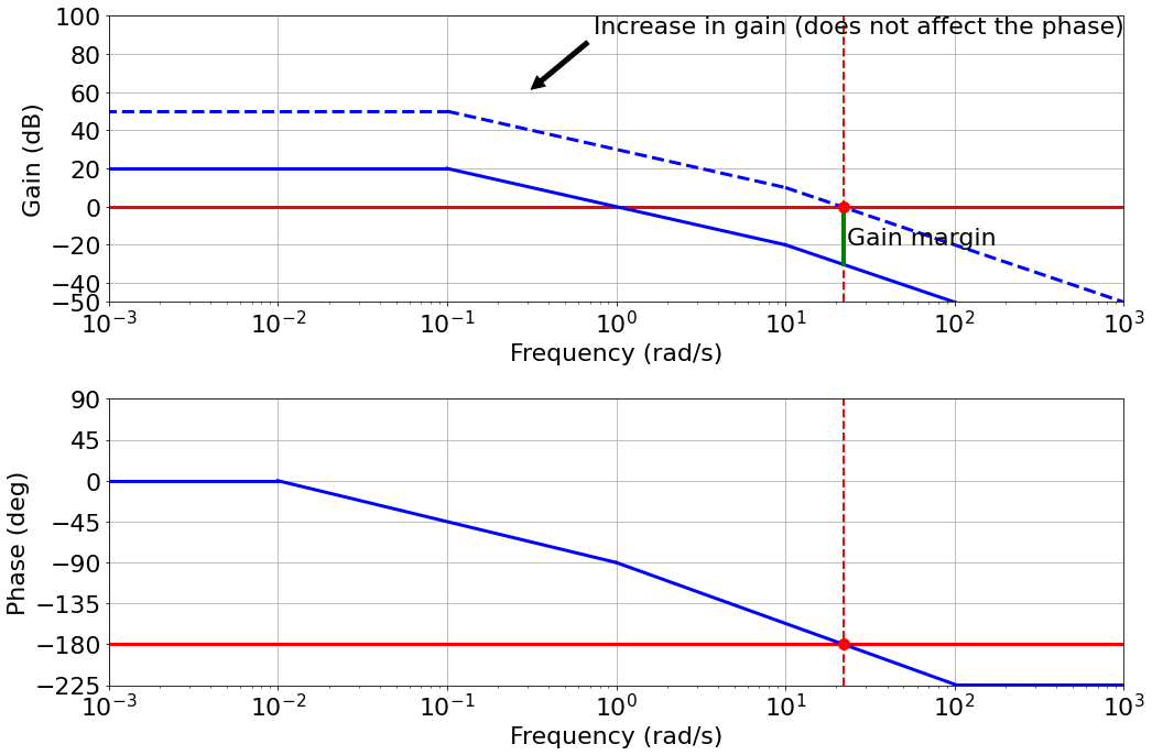
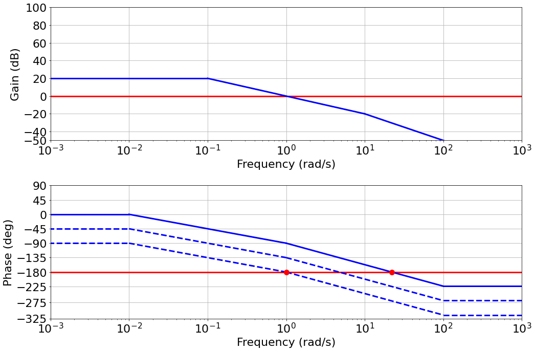
• Gain and Phase margin: extra gain or phase that we have available before the system starts to oscillates or become unstable

• Robustness of the system

• Makes it possible to quantify how stable a system is

  • Systems (or designs) that have less margin could be considered as being "less" stable: smaller variations in the system could lead to instability

• We want our controller to be robust to these because we cannot know our system perfectly and hence we need margins.

• The more uncertainty we have the more margin we should design in.

• Gain margin: The gain required to cross the 0dB line at the frequency where phase is $-180^o$
• Phase margin: how much phase delay takes to make $-180^o$ phase at the 0 $dB$ gain frequency.

• Uncertainty in one specific parameters can affect you more than you think.

Loop analysis and loop shaping

Feedback Goals

• Stability of the closed loop system
• Performance while tracking inputs
  • tracking error, typically specified in terms of steady state error to specific inputs:
    • e.g., error to step inputs less than $5\%$
  • behaviour of the transient, typically specified in terms of bandwidth, rise time, settling time, damping ratio, overshoot (these are requirements for the transfer function between $Y$ and $Y_{ref}$).
• Robustness to noise measurement and disturbances

• One advantage of the Nyquist stability theorem is that it is based on the loop transfer function $L = GR$,
• Easy to see how the controller influences the loop transfer function.
• Loop shaping: Choose a compensator that gives a loop transfer function with a desired shape.

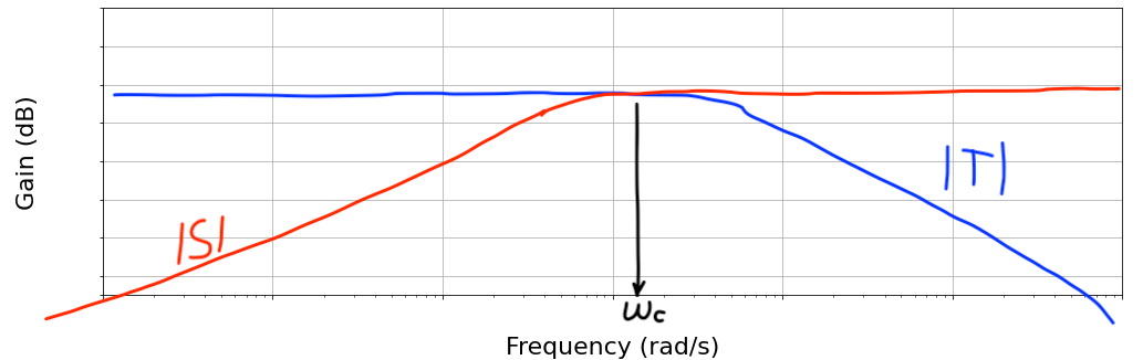
Sensitivity and Complementary Sensitivity Functions

We want to design $R$ so that all transfer functions have good properties

• tracking (at freq. where this is important)
• disturbance rejection (at freq. where this is important)
• noise attenuation (at freq. where this is important)

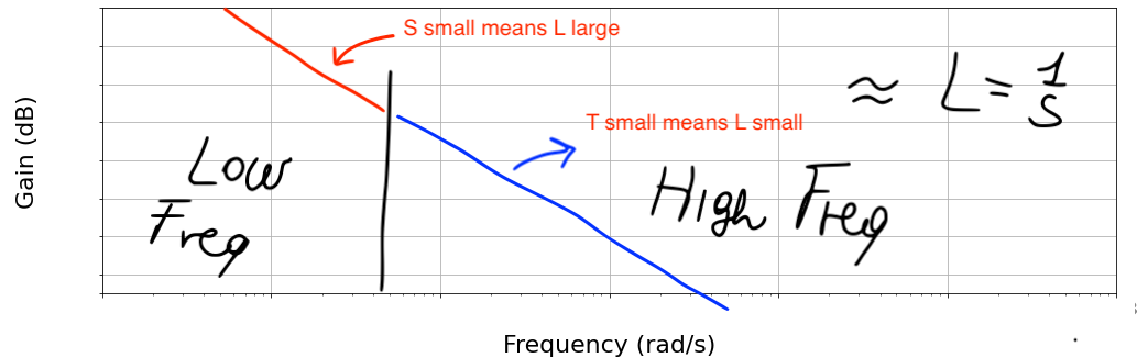
• $L(s)=G(s)R(s)$
• $S(s)=\frac{1}{1+L(s)}$
• $T(s)=\frac{L}{1+L(s)}$

• Is a trial-and-error procedure
• We typically start with a Bode plot of the process transfer function $G$
• Choosing the gain crossover frequency $\omega_{gc}$ is a major design decision: a compromise between attenuation of load disturbances and injection of measurement noise
• Finally shape the loop transfer function by changing the controller gain and adding poles and zeros to the controller transfer function
• The controller gain at low frequencies can be increased by so-called lag compensation, and the behavior around the crossover frequency can be changed by so-called lead compensation.

Nominal sensitivity peak $$ M_s = \max_{0 \leq \omega \leq \infty} | S(j\omega) | = \max_{0 \leq \omega \leq \infty} \Big| \frac{1}{1+G(j\omega)R(j\omega)} \Big| $$

• $M_s$ gives us an indication of how far $L$ is from -1

Relationship between loop function harmonic response and closed loop

• Relationship between the harmonic response of the loop transfer function $L(j\omega)$ and the closed loop $H(j\omega)$

$$ |H(j\omega)| = \frac{|L(j\omega)|}{|1+L(j\omega)|} = \frac{|L(j\omega)|}{\sqrt{1+|L(j\omega)|^2}} $$

• Translation of design requirements into requirements on the Bode plot of the loop funtion (barriers)
• The "barriers" on the Bode plots are there to help us shape the desired harmonic response of the loop function
• The controller is designed so that the loop function always stays within the admissible regions

Root Locus

• System with multiple known parameters, and one unknown or varying parameter (K)
• Changing $K$ changes the locations of the poles
• How to design a system that meets the requirements:
  • What value of $K$ should I choose to meet the requirements (i.e., that places the poles at the correct location in the $s$ plane)

• What is the effect of variations on a control system that has been already designed:

  • How sensitive is the system to a value of $K$ that is slightly different than what we have estimated (or predicted).

• Rules to sketch the root locus

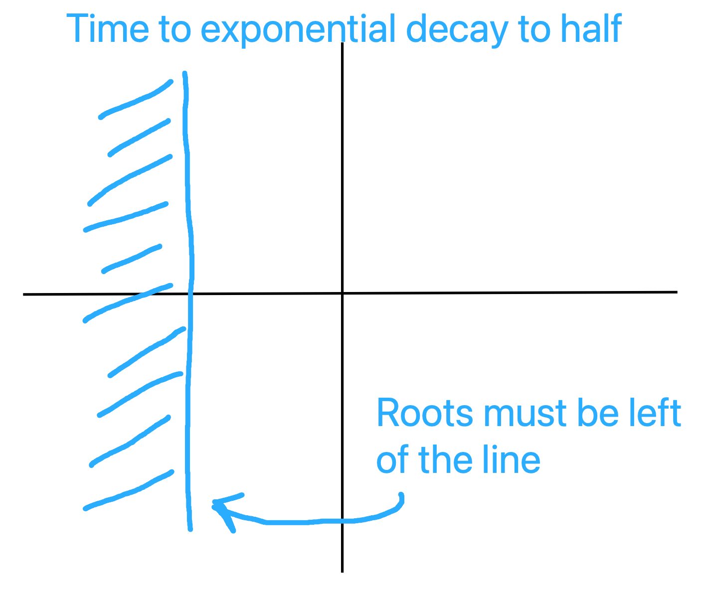
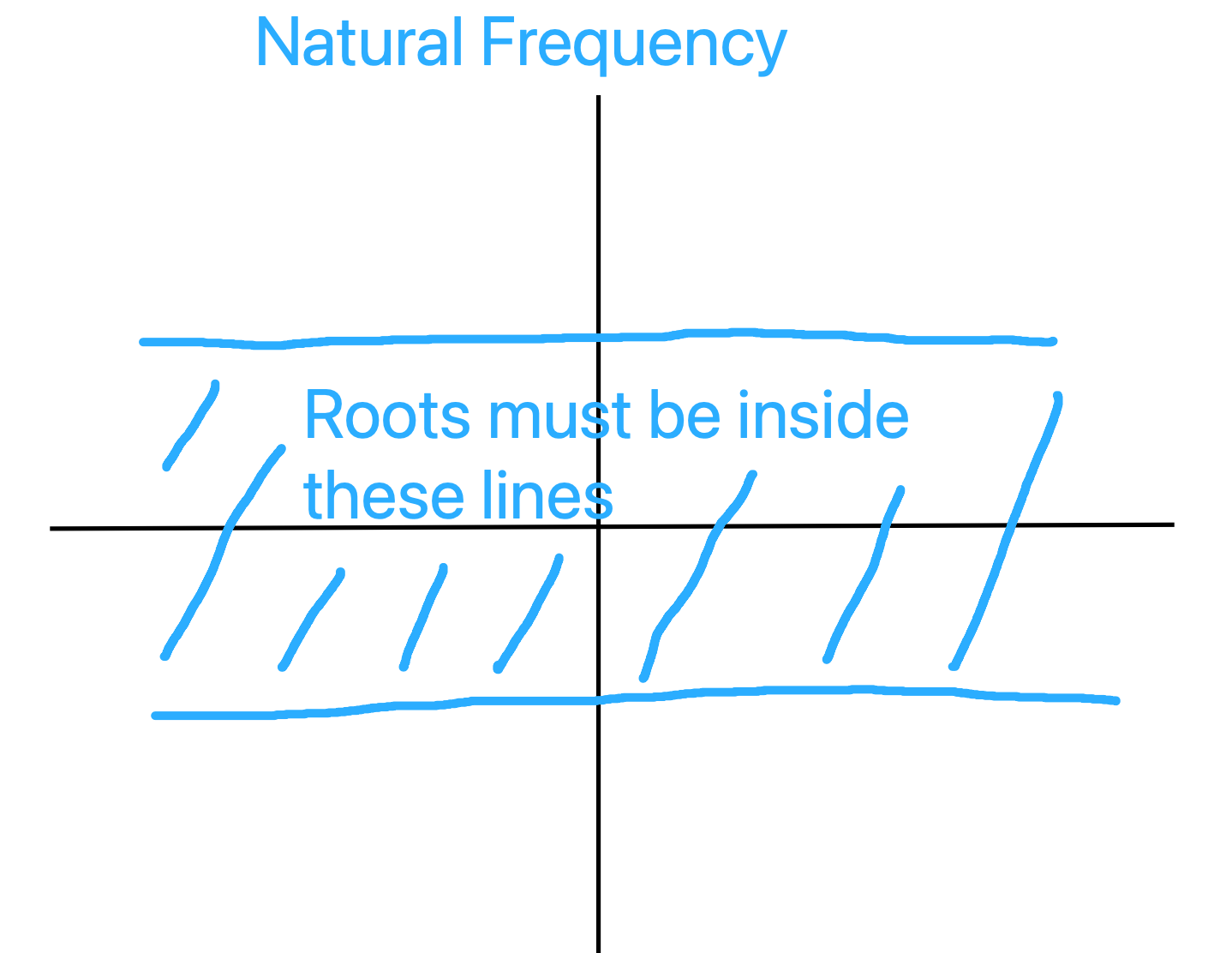
• Translate requirements into s-plane requirements:

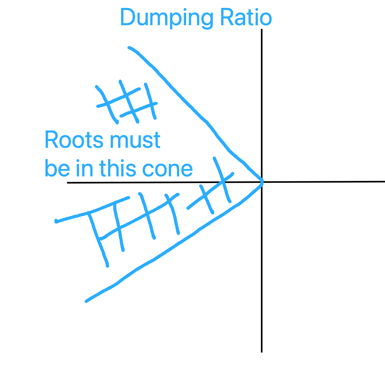• The angle condition: $\angle (G(s)) = (2n + 1)\pi$

• The magnitude condition: $|KG(s)|=1$

Phase Lead/Phase Lag Compensators

• A lead compensator can increase the stability or speed of reponse of a system;
• A lag compensator can reduce (but not eliminate) the steady-state error.

$$ R(s) = \frac{\frac{s}{w_z}+1}{\frac{s}{w_p}+1} = \frac{w_p}{w_z}\frac{s + w_z}{s + w_p} $$

Lead compensator:

• $w_z < w_p$
• $K=\frac{w_p}{w_z}$ (gain)

Lag compensator

• $w_z > w_p$
• $K=\frac{w_p}{w_z}$ (gain)

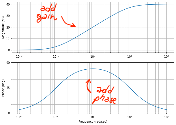
• Multiplying the two T.F. together means adding everything together on the Bode plot
• Lead/Lag compensator:
  • Behaves like a real zero early on, at low frequency
  • Until the real pole pulls it back at high frequency
  • See blue line for its approximate representation

• Using the root locus and Bode plots to place the zero and pole

PID Controllers

• PID = Proportional-Integral-Derivative

  • Describes how the error term is treated before being sum and sent into the plant

• It is a simple and effective controller in a wide range of applications

• Majority of controllers in industrial applications are PIDs

The general structure of a PID controller is:

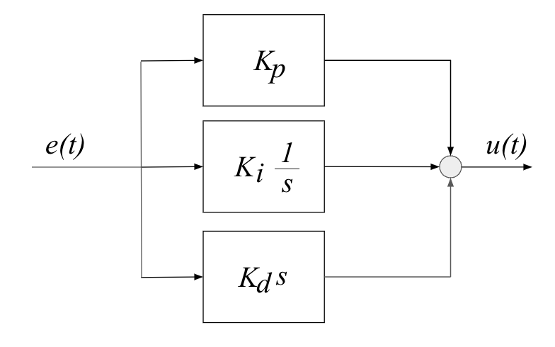• The three gains $K_p, K_i, K_d$ are adjustable and can be tuned to the specific application
• Varying $K_p, K_i, K_d$ means adjusting how sensitive the system is across the three paths

• Ziegler Nichols tuning rules
• Practical problems:
  • Derivative is sensitive to noise
    • Filtering and Set Point Weighting
  • If the integral of the error grows too much, the control output might hit actuation limits
    • Integral windup: Initializing the controller integral to a desired value or zeroing the integral value every time the error is equal to, or crosses zero reduces the problem.

• Solving the Cruise Control Problem deploying a PID controller on a car

Fin