import numpy as np
import matplotlib.pyplot as plt
import control

Standard Feedback loop

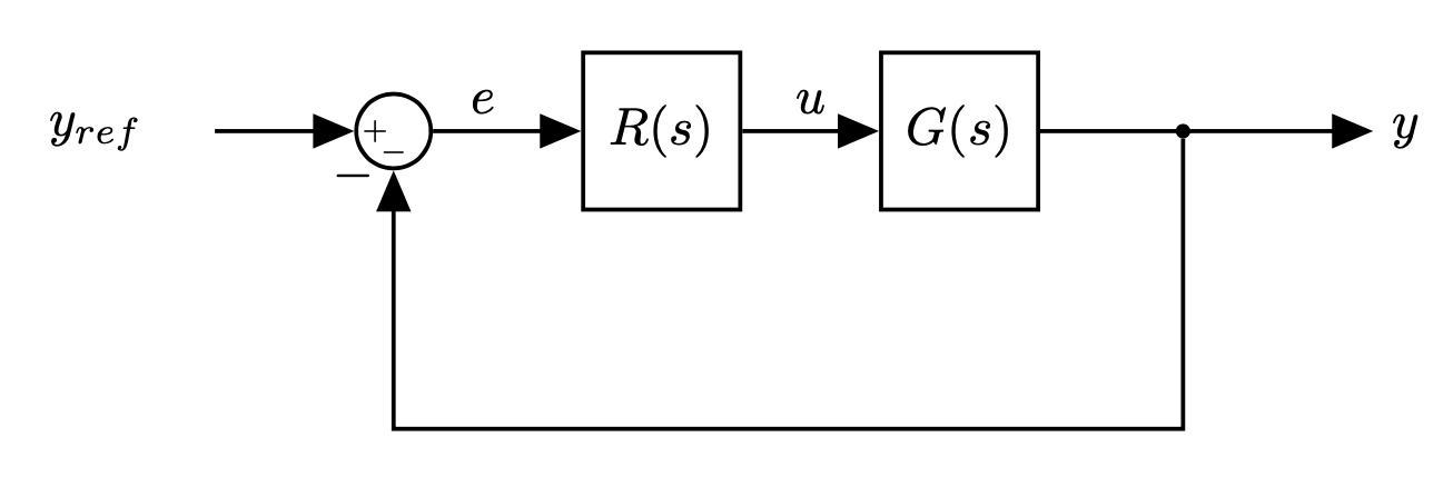Controller $R(s)$ :

Converts the error term into an actuator command
We are free to choose any control scheme we like.
As long as the closed loop performance of the system meets our requirements

Note: controller = compensator

Lead and lag compensators are used quite extensively in control.
A lead compensator can increase the stability or speed of reponse of a system;
A lag compensator can reduce (but not eliminate) the steady-state error.
Depending on the effect desired, one or more lead and lag compensators may be used in various combinations.
Lead, lag, and lead/lag compensators are usually designed for a system in transfer function form.

Phase Lead

What is phase lead

t = np.arange(0, 10, 0.1)
plt.plot(t, np.sin(t), color='r', label='sin');
plt.plot(t, np.cos(t), color='b', label='cos');
plt.legend();
plt.grid()

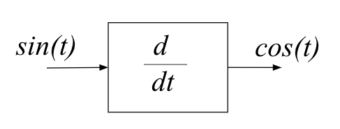
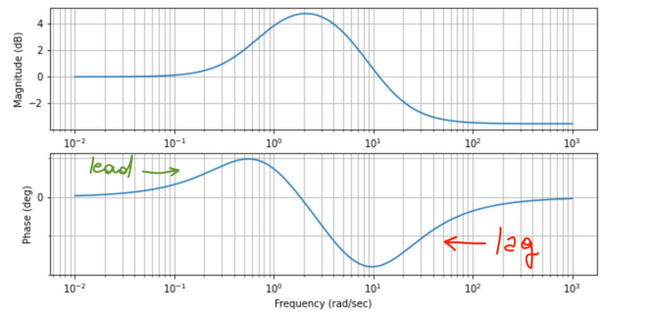
The $cos$ signal is ahead of the $sin$ signal by $90$ deg
The output leads the input by 90 deg

We can plot the Bode plots:

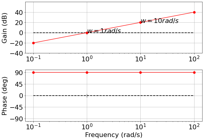Differentiation gives positive phase
Integration gives negative phase (Mirrors the derivative plot)
A zero in a transfer function adds phase
A pole in a transfer function subtracts phase
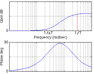
Lead compensator: adds phase (at least in some frequency range of interest)
Lag compensator: subtracts phase (at least in some frequency range of interest)

Equations

Lead compensator

R(s) = \frac{\frac{s}{w_z}+1}{\frac{s}{w_p}+1} = \frac{w_p}{w_z}\frac{s + w_z}{s + w_p}

one real pole and one real zero
$w_z < w_p$
$K=\frac{w_p}{w_z}$ (gain)
We can take care of the gain easily (e.g., using the root locus method)

Lag compensator

R(s) = \frac{\frac{s}{w_z}+1}{\frac{s}{w_p}+1} = \frac{w_p}{w_z}\frac{s + w_z}{s + w_p}

one real pole and one real zero
$w_z > w_p$
$K=\frac{w_p}{w_z}$ (gain)

Bode plot: Lead Compensator

R(s) = \frac{w_p}{s + w_p}\frac{s + w_z}{w_z}

Let's look at the zero-pole contribution separately:

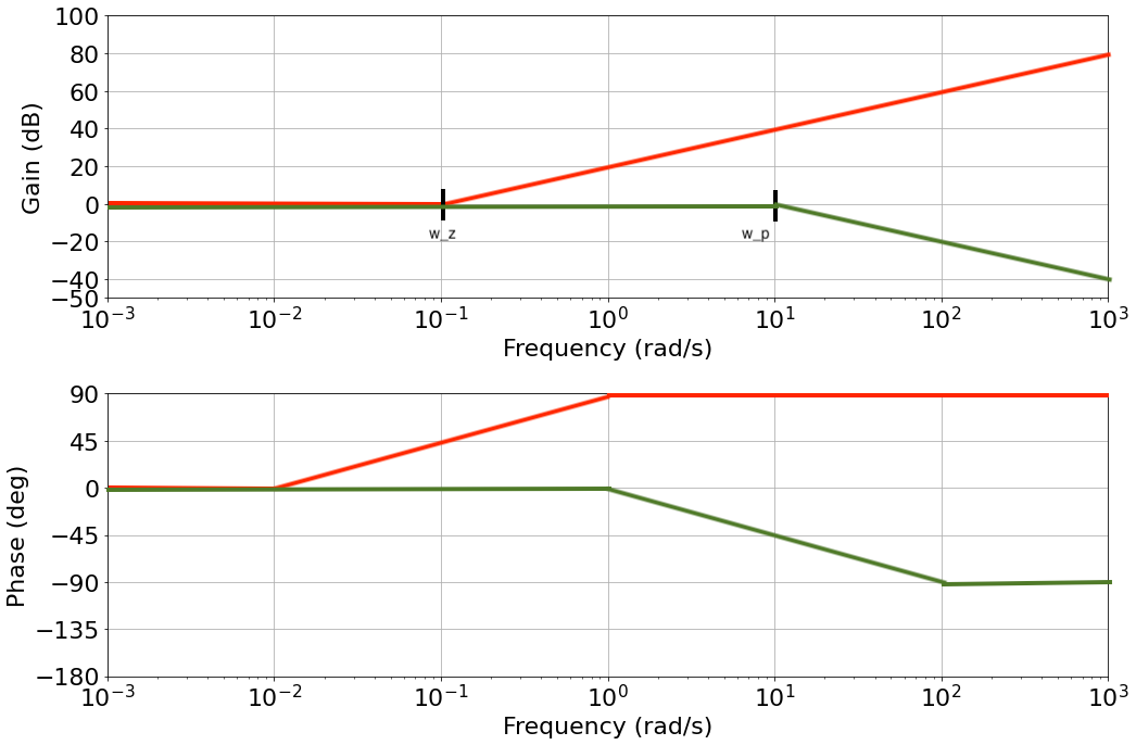The zero adds 90 deg and amplifies high frequencies
The pole subtracts 90 deg and attenuates high frequencies

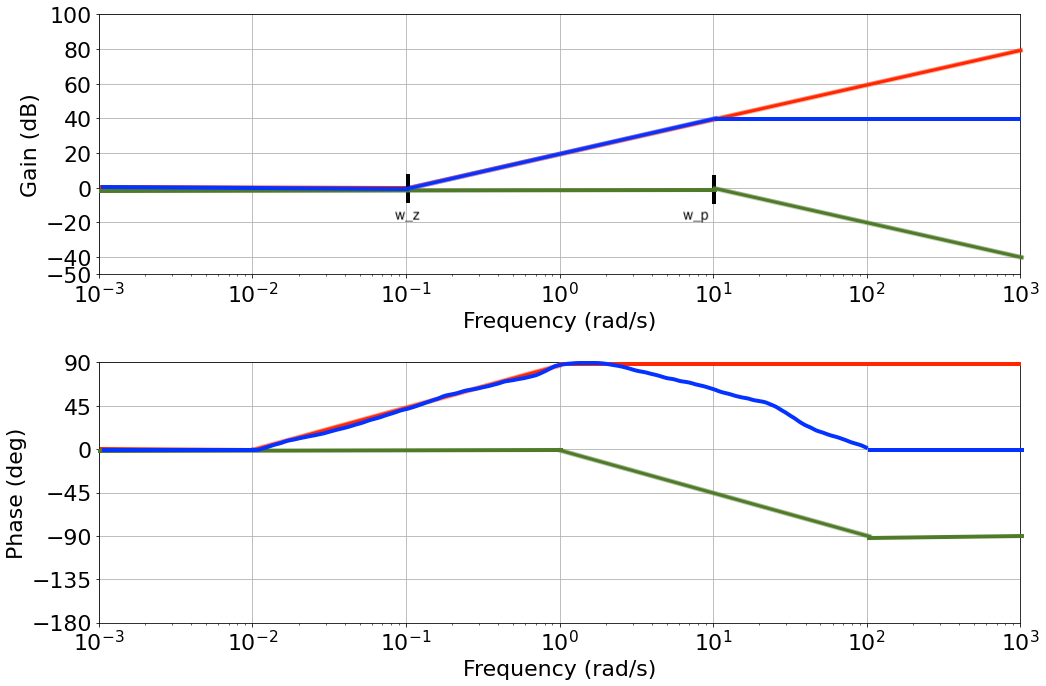
Multiplying the two T.F. together means adding everything together on the Bode plot
Lead/Lag compensator:
- Behaves like a real zero early on, at low frequency
- Until the real pole pulls it back at high frequency
- See blue line for its approximate representation

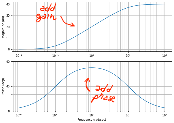
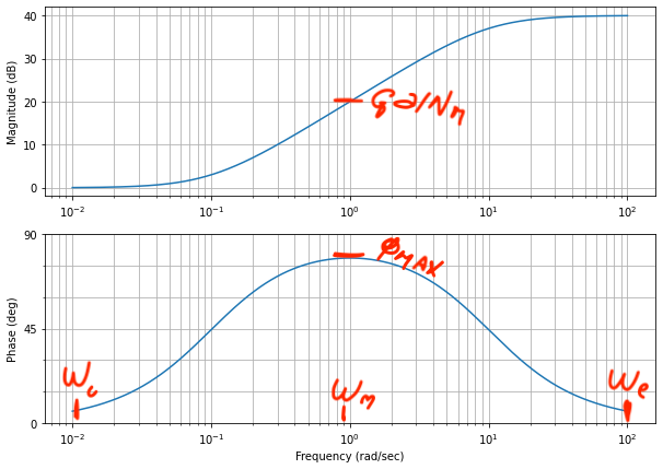
Note:

A lead compensator increases the gain at high frequency (but less than a real zero would do)
This means that it is less noisy than a derivative controller on its own
A lead compensator adds phase between the two corner frequencies and no phase outside
Moving the two frequency means we can change where we add our phase

Example

Let's see an example:

w_z = 1
w_p = 10

s = control.tf([1, 0], [1])

R_s = w_p/(s+w_p)*(s+w_z/w_z)

We can plot the zero (blue) and the pole (orange) parts together with the combined Bode plot (green):

fig, axs = plt.subplots(1, figsize=(10,5))

# zero (blue)
control.bode_plot((s+w_z)/w_z, dB=True, omega_limits = [0.1, 100], wrap_phase =True);
# pole (orange)
control.bode_plot(w_p/(s+w_p), dB=True, omega_limits = [0.1, 100], wrap_phase =True);

# compensator (green)
control.bode_plot(R_s, dB=True, omega_limits = [0.1, 100], wrap_phase =True);

# Note: If wrap_phase is True the phase will be restricted to the range [-180, 180) (or [-\pi, \pi) radians)

What happens when we move the zero closer to the pole?

w_z = 5
w_p = 10

fig, axs = plt.subplots(1, figsize=(10,5))

# zero (blue)
control.bode_plot((s+w_z)/w_z, dB=True, omega_limits = [0.1, 100], wrap_phase =True);
# pole (orange)
control.bode_plot(w_p/(s+w_p), dB=True, omega_limits = [0.1, 100], wrap_phase =True);

# compensator transfer function (green)
R_s = w_p/(s+w_p)*(s+w_z)/w_z
control.bode_plot(R_s, dB=True, omega_limits = [0.1, 100], wrap_phase =True);

Still a phase lead is present, but much smaller
What happens if the zero is right on top of the pole?

if $w_p$ < $w_z$ we obtain a lag compensator

w_z = 50
w_p = 10

fig, axs = plt.subplots(1, figsize=(10,5))
# zero
control.bode_plot((s+w_z)/w_z, dB=True, omega_limits = [1, 1000], wrap_phase =True);
# pole
control.bode_plot(w_p/(s+w_p), dB=True, omega_limits = [1, 1000], wrap_phase =True);

# compensator transfer function
R_s = w_p/(s+w_p)*(s+w_z)/w_z
control.bode_plot(R_s, dB=True, omega_limits = [1, 1000], wrap_phase =True);

The zero affects the system at higher frequency
The system behaves like a real pole at lower frequency
Until the zero comes into effect and "cancels" the pole at higher frequency
This add lag to the system

Note: The sama transfer function structure can produce phase lead or lag, adjusting the relative position of the pole and the zero

Lead/Lag compensators

Design a compensator that uses both a lead and a lag compensator:

R(s) = \frac{\frac{s}{w_z}+1}{\frac{s}{w_p}+1} \frac{\frac{s}{w_{z1}}+1}{\frac{s}{w_{p1}}+1} = \frac{w_p}{w_z}\frac{s + w_z}{s + w_p}\frac{w_{p1}}{w_{z1}}\frac{s + w_{z1}}{s + w_{p1}}

w_z = .5
w_p = 1

R_Lead = w_p/(s+w_p)*(s+w_z)/w_z

# Lag compensator
w_z1 = 15
w_p1 = 5

R_Lag = w_p1/(s+w_p1)*(s+w_z1)/w_z1

Plot the pole zero map for the Lead compensator:

control.pzmap(R_Lead);

Plot the pole zero map for the Lag compensator:

control.pzmap(R_Lag);

We construct the Lead-Lag compensator:

R_LL = R_Lead*R_Lag

And we can plot the Bode Plot to see what the phase does:

fig, axs = plt.subplots(1, figsize=(10,5))
control.bode_plot(R_LL, dB=True, omega_limits = [.01, 1000], wrap_phase =True);

This compensator is leading at low frequency, and lagging at higher frequency

Designing a Lead Compensator with the Root Locus

Let's consider our control loop again:

We have a model of our plant $G(s)$
- we are given a transfer function
- we have identified the model
Design requirements - performance goal:
- Stability
- Rise time
- Settling time
- Max Overshoot
- Damping ratio
- Gain/Phase margin
$G(s)$ alone does not meet our requirements
We need to design the controller $R(s)$

How do we choose $R(s)$ ?

Let's consider:

G(s) = \frac{1}{(s+2)(s+4)}

What is the Root Locus of $G(s)$ ?

s = control.tf([1, 0],[1])

G_s = 1/((s+2)*(s+4))

fig, axs = plt.subplots(1, figsize=(10,5))
control.rlocus(G_s);

What if we had a Lead compensator?
How does the root locus change?

Let's choose, arbitrarily, a Lead compensator ( $w_z < w_p$ ):

R(s) = \frac{(s+5)}{(s+6)}

Let's see how it looks like with Python:

We define the controller:

R_s = (s+5)/(s+6)

Plot the Root Locus:

fig, axs = plt.subplots(1, figsize=(10,5))
control.rlocus(G_s*R_s);

With a lead compensator:

We have moved the asynmptotes further into the left half plane
Increasing the gain $K$ the close loop poles would be more to the left: we have added stability to the system

How does this help us?

When we use the root locus method we typically know where we would like our dominant closed loop poles to be so that we meet our requirements
With the root locus method, we first convert our requirements into pole locations

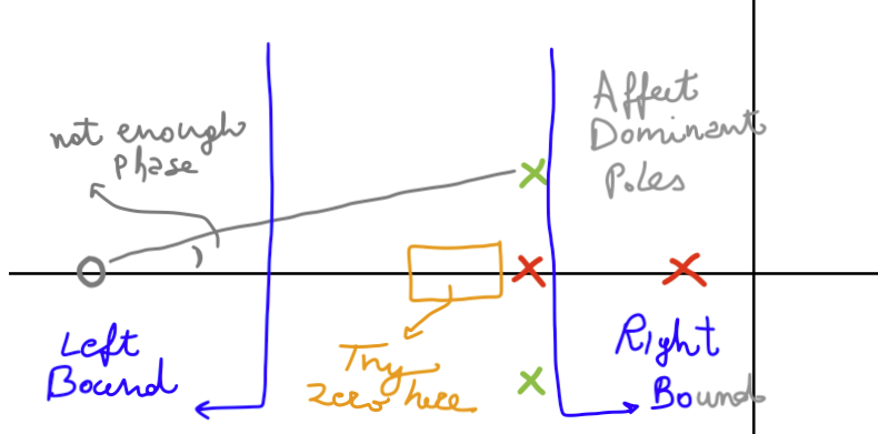
We need a lead compensator if we need to move our poles to the left of where our current (uncompensated) poles are
We need a lag compensator if we need to move our poles to the right of where our current (uncompensated) poles are
If the root locus already goes through the desired locations, we only need to choose the correct gain
- Note: we could still have a steady state error problem, but we know how to fix this already

Given desired poles, solving for the compensator becomes a trigonometry problem:
To be part of the Root Locus: $\sum{\angle Poles} - \sum{\angle Zeros} = 180^o$

For example, for our system we saw that the root locus is:

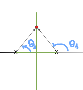There are no zeros (so we do not need to subtract)
The sum of $\theta_1+\theta_2$ =180 because that point is part of the root locus

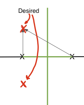
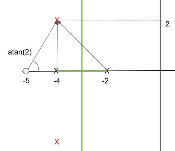
Given our system: $G(s) = \frac{1}{(s+2)(s+4)}$

If we want poles:

$s_d = -4 \pm 2j$

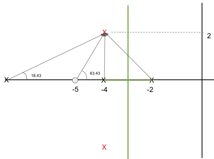
And if we sum up all the angles: $90+(90+\theta)$ = $90+(90+45)$ = 225

since $\theta = \tan^{-1}(2/2) = \tan^{-1}(1) = 45$

And of course, this is not on the Root Locus.

To have it on the Root Locus, we need to remove 45 deg of phase
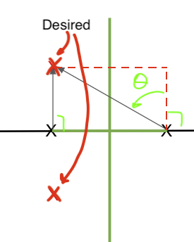
Using a phase lead compensator we can do it adding a single pole and a single zero:

225 + (\theta_p - \theta_z) = 180

$(\theta_p - \theta_z)$ is our lead compensator

If we pick a zeros at -5
- $\theta_z= 63.43 ^o$
The pole must go into one specific location:
- $\theta_p=180-225+63.43=18.43$

The compensator for this particular problem is:

R(s) = \frac{s+5}{s+10.015}

%matplotlib notebook
R_s = (s+5)/(s+10.015)
fig, axs = plt.subplots(1, figsize=(7,7))
control.rlocus(G_s*R_s);

One more step:

We need to calculate the gain that moves the poles in closed loop where we want them

\frac{KG(s)R(s)}{1+KG(s)R(s)}

We can then find:

K = \frac{-1}{1+G(s)R(s)}\Big|_{s=-4 + 2 j} \approx 16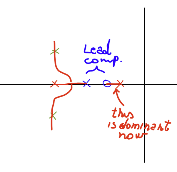

Choosing the first zero

No hard and fast rule
We need to have enough negative angle to bring the sum to 180 deg
Pay attention not to interfere with your dominat poles
- For example, if you had:

We can then sketch bounds:

</tr> </table>

Rule fo thumb: place your zero at or closely to the left of the second real axis open loop pole

Does not guarantee that overshoot requirements will be met
Trial and error might be needed
With higher order systems, might be difficult to predict where other non-dominant poles go: we must avoid making them unstable
Faster responding system means responding to noise as well.

Designing a Lag Compensator with Root Locus

R(s) = \frac{\frac{s}{w_z}+1}{\frac{s}{w_p}+1} = \frac{w_p}{w_z}\frac{s + w_z}{s + w_p}

one real pole and one real zero
$w_z > w_p$
$K=\frac{w_p}{w_z}$ (gain)

We can re-write the above equation as:

R(s) = \frac{\tau_z s + 1}{\tau_p s + 1}

The transfer function has the same structure
We can use the same design technique that we saw for the Lead Compensators

With a Phase Lag compensator we can move our dominant poles closer to the imaginary axis
This is however not the main reason Lag Compensators
Lag Compensators are useful to address steady state errors
- e.g., error to the step input
- improve steady state errors, without changing the position of the dominant poles (they are already where we need them)
- this means we do not want shape the root locus very much

How does a lag compensator reduce $E_{ss}$

Where: $G(S) = \frac{N(s)}{D(s)}$

and our Lag compensator is:

R(s) = \frac{s-z}{s-p}

and the input is $U(s)$ .

The steady state error for the uncompensated system is:

E_{ss} = \lim_{s\rightarrow0} s \cdot \frac{U(s)}{1+\frac{N(s)}{D(s)}}

For a step input: $U(s)=\frac{1}{s}$

\Rightarrow E_{ss} = \lim_{s\rightarrow0} s \cdot \frac{U(s)}{1+\frac{N(s)}{D(s)}} = \frac{D(0)}{D(0)+N(0)}

The steady state error for the compensated system is:

E_{ss} = \lim_{s\rightarrow0} s \cdot \frac{U(s)}{1+\frac{N(s)(s-z)}{D(s)(s-p)}}

For a step input: $U(s)=\frac{1}{s}$

\Rightarrow E_{ss,c} \lim_{s\rightarrow0} s \cdot \frac{U(s)}{1+\frac{N(s)(s-z)}{D(s)(s-p)}} = \frac{D(s)(s-p)}{D(s)(s-p)+N(s)(s-z)}\Big|_{s\rightarrow0} = \frac{D(0)p}{D(0)p+N(0)z}

\frac{z}{p} = \frac{D(0)-E_{ss,c}D(0)}{E_{ss,c}N(0)}

We can choose $E_{ss,c}$ and have the corresponding $\frac{z}{p}$
To have $E_{ss,c}=0$ , $\frac{z}{p} \rightarrow \infty$
We can only reduce the steady state error and not eliminate it. We need to change the system type to eliminate it

Rule fo thumb: place your zero at or closely to the left of the second real axis open loop pole

Does not guarantee that overshoot requirements will be met
Trial and error might be needed
With higher order systems, might be difficult to predict where other non-dominant poles go: we must avoid making them unstable
Faster responding system means responding to noise as well.

Designing a Lag Compensator with Root Locus

R(s) = \frac{\frac{s}{w_z}+1}{\frac{s}{w_p}+1} = \frac{w_p}{w_z}\frac{s + w_z}{s + w_p}

one real pole and one real zero
$w_z > w_p$
$K=\frac{w_p}{w_z}$ (gain)

We can re-write the above equation as:

R(s) = \frac{\tau_z s + 1}{\tau_p s + 1}

The transfer function has the same structure
We can use the same design technique that we saw for the Lead Compensators

With a Phase Lag compensator we can move our dominant poles closer to the imaginary axis
This is however not the main reason Lag Compensators
Lag Compensators are useful to address steady state errors
- e.g., error to the step input
- improve steady state errors, without changing the position of the dominant poles (they are already where we need them)
- this means we do not want shape the root locus very much

How does a lag compensator reduce $E_{ss}$

Example

G(s) = \frac{5s^2+6s+2}{4s^2+s+3}

Goal: reduce steady state error $E_{ss, c}=0.1$

\frac{z}{p} = \frac{D(0)-E_{ss,c}D(0)}{E_{ss,c}N(s)} = \frac{3-E_{ss, c}\cdot 3}{E_{ss, c}\cdot2} = \frac{3-0.1\cdot3}{0.1\cdot2} = 13.5

We know the zero/pole ratio
Where do we place them?
E.g., $z=-0.1$ , $p=-1.35$ or $z=1$ , $p=13.5$ would work

Remember that the Root Locus is where the angles of poles (+) and zeros (-) add to 180 degrees

We do not want to move the location of our roots too much when using a Lag compensator
The the angle of the poles and zeros of the compensator should be very small (no Root Locus shaping):

\theta_p - \theta_z \approx 0

Meeting the condition above while keeping the desired $\frac{z}{p}$ is much easier if we place the zero and pole very close to the imaginary axis
Practical constraints means you cannot move them too close (resistors and capacitors limits)

Rule of thumb: the location of the zero is approximately 50 times closer to the imaginary axis as the closer dominant pole

E.g.,

dominant poles at $-1\pm \text{Imag} j$
zero at $-1/50=0.02$
pole at $\Big(\frac{z}{p}\Big)_{des} = \frac{0.02}{p}$

Example

G(s) = \frac{1}{(s+1)(s+3)}

With a Lead compensator to meet stability and rise time requirements $R(s) = \frac{16(s+4)}{(s+9)}$

In this case: $E_{ss} = \frac{D(0)}{D(0)+N(0)} = \frac{9\cdot3\cdot1}{9\cdot3\cdot1+16\cdot4}\approx 0.3$

Requirement: $E_{ss} =0.1$

\frac{z}{p} = \frac{D(0) -E_{ss} D(0)}{E_{ss} N(0)} = \frac{9\cdot3\cdot1 - 0.1\cdot9\cdot3\cdot1}{0.1\cdot16\cdot4} \approx 3.8

Dominant poles: $s_{1,2} = -3\pm-2j$

The zero goes to $\frac{-3}{50} = -0.06$
The Pole goes to $3.8 = \frac{-0.06}{p} \Rightarrow p = -0.6/3.8 = -0.016$

Lag compensator: $R(s) = \frac{s+0.06}{s+0.016}$

We can have the Lag compensator in series with a Lead compensator

Exercise:

Plot the step response and the impulse respose of the uncompensated and compensated system

s = control.tf([1, 0],[1])

sys_u = 1/((s+1)*(s+3))*(16*(s+4)/(s+9))
print('sys_u', sys_u)

sys_c = 1/((s+1)*(s+3))*(16*(s+4)/(s+9))*(s+0.06)/(s+0.016)
print('sys_c', sys_c)

sys_u 
       16 s + 64
------------------------
s^3 + 13 s^2 + 39 s + 27

sys_c 
           16 s^2 + 64.96 s + 3.84
---------------------------------------------
s^4 + 13.02 s^3 + 39.21 s^2 + 27.62 s + 0.432

t_u, yout_u = control.step_response(control.feedback(sys_u, 1), T=100)
t_c, yout_c = control.step_response(control.feedback(sys_c, 1), T=100)

fig, ax = plt.subplots(1, figsize=(10,7))

plt.plot(t_u, yout_u, color='b', label='uncompensated');
plt.plot(t_c, yout_c, color='r', label='compensated');
plt.grid();
plt.legend();
plt.yticks(np.arange(0, 1, 0.1));

As expected: the uncompensated system has $E_{ss} = 0.3$
The compensated system has $E_{ss} = 0.1$
Settling time does not change very much, as desired

We can see this better looking at the impulse response

t_u, yout_u = control.impulse_response(control.feedback(sys_u, 1), T=3)
t_c, yout_c = control.impulse_response(control.feedback(sys_c, 1), T=3)

fig, ax = plt.subplots(1, figsize=(10,7))

plt.plot(t_u, yout_u, color='b', label='uncompensated');
plt.plot(t_c, yout_c, color='r', label='compensated');
plt.grid();
plt.legend();
plt.yticks(np.arange(0, 1.5, 0.1));

This confirmes that we did not change the position of the dominant poles very much

Designing a Lead Compensator with the Bode Plot

Let's consider our control loop again:

Compensator: Lead compensator, so we need to select one pole and one zero

First: Convert requirements to frequency domain requirements if needed
- Gain/Phase margin
- Bandwidth
- Gain crossover frequency
- Zero-frequency magnitude or DC Gain
- Steady-state error

A phase-lead compensator can also be designed using a frequency response approach. A lead compensator in frequency response form is given by the following transfer function:

Lead(s) = \frac{a\tau s + 1}{\tau s + 1}

with $a>1$ (when $a<1$ we would have a lag compensator).

Note that the previous expression is equivalent to the form (which we used for the Root Locus):

Lead(s) = K\frac{s + w_z}{s + w_p}

when $w_p =\frac{1}{\tau}$ , $w_z = \frac{1}{a\tau}$ , and $K = a$ .

In frequency response design, the phase-lead compensator adds positive phase to the system over the frequency range $\frac{1}{a\tau}$ to $\frac{1}{\tau}$ .

And a Bode plot of a phase-lead compensator $Lead(s)$ has the following form:

The two corner frequencies are at $\frac{1}{a\tau}$ and $\frac{1}{\tau}$
Note the positive phase that is added to the system between these two frequencies.
Depending on the value of $a$ , the maximum added phase can be up to 90 degrees
If you need more than 90 degrees of phase, two lead compensators in series can be employed.

Example

G(s) = \frac{1}{0.2s+1}

System requirements

Steady state error < 0.02 to a unit ramp input
Phase margin $> 48$ deg

For a ramp unit (assuming a stable system):
- we need at least a type 1 system to have a finite error (single pole at the origin)
- we need at least a type 2 system to have a zero error

Note we cannot meet our requirements with a lead compensator alone. It does not have a pole at the origin

Our controller needs to have this structure to start from $R(s) = K\frac{1}{s}$

and now we can add the lead compensator to deal with the phase margin.

It is always better to start from the type of the system: adding a pole at the origin will affect your phase.
Given that a single pole at the origin is enough, we will not add a second one
- Adds complexity
- Might reduce stability
- Do not overdesign!

Choose the gain to meet $e_{ss} < 0.02$

For an input $U(s)$ :

e_{ss} = \lim_{s\rightarrow0}sE(s) = s \frac{1}{1+G_F(s)}U(s)

where, in this case:

G_F(s) = G(s)K\frac{1}{s}

Ramp = \frac{1}{s^2}

If we plug in the numbers:

e_{ss} = \lim_{s\rightarrow0}sE(s) = s \frac{1}{s^2}\frac{0.2s^2+s}{0.2s^2+s+K+1} < 0.02 \Rightarrow K > 49

We can then choose:

R(s) = 50\frac{1}{s}

Let's now draw the Bode plot:

Bring the system in the Bode form
Sketch the Bode Diagram for each individual part
Add them all up

lead-lag-compensator-bode-example-result

Let's check it with Python

s = control.tf([1, 0], [1])
G_s = 1/(0.2*s+1)
R_s = 50/s

fig, ax = plt.subplots(1, figsize=(10,7))
control.bode_plot(G_s*R_s, dB=True);

[gm, pm, _, pm_f] = control.margin(G_s*R_s)

print('Phase margin: deg', pm, 'at rad/s', pm_f)

Phase margin: deg 17.964235916371393 at rad/s 15.421164188583809

We do not respect our phase margin requirement $18<48$

A lead compensator adds phase for a specific frequency range
We also add gain, which means we move the crossover frequency to higher frequency

To determin how much phase let's look at the lead compensator equations, which we can re-write in this form to highlight the relative relationship between the pole and the zero:

Lead(s) = \frac{a\tau s + 1}{\tau s + 1}

In this form, the steady state gain is 1 (0 dB). Does not affect the steady state we already determined.
$a > 1$ to be a lead compensator
$a < 1$ is a lag compensator

From the equation above it is easy to verfy that the following equations can be used to determine significant points of the response:

Upper cutoff frequency $w_u = \frac{1}{a\tau}$

gain starts to increase

Lower cutoff frequency

w_l = \frac{1}{\tau}

gain starts to flatten out

Max phase (obtained at the center frequency $w_m$ )

\Phi_{max} = \sin^{-1} \Big( \frac{a-1}{a+1} \Big)

Freq at Max phase $w_{m} = \frac{1}{\tau\sqrt{a}}$

Gain at Max phase $Gain_{m} = \sqrt{a}$

Choosing $a$ and $\tau$ :

Choose the maximum phase you would like to add $\Phi_{max}$ and solve for $a$
Choose the frequency $w_{m}$ where you would like to add $\Phi_{max}$ and solve for $\tau$

We would get a lower phase increase
Trial and error is an option
- Add a safety factor (e.g., 15 deg)

Let's go back to our design

We need 30 deg more at 15 rad/s (from 18 to 38)
We add some safety factor:

$\Phi_{max} = \sin^{-1} \Big( \frac{a-1}{a+1} \Big) = 37 \Rightarrow a=4$

Freq at Max phase $w_{m} = \frac{1}{\tau\sqrt{a}} = 22.2 rad/s \Rightarrow \tau=0.022$

Final controller:

R(s) = 50\frac{1}{s}\frac{0.088s+1}{0.022s+1}

And we should verify that we obtain the desired phase margin plotting the Bode plot.

Let's plot the Bode plots for

the initial controller (in blue) $R(s) = G(s)\frac{50}{s}$
the final lead compensator (in orange) $R(s) = 50\frac{1}{s}\frac{0.088s+1}{0.022s+1}$

s = control.tf([1, 0], [1])
G_s = 1/(0.2*s+1)
R_s = 50/s*(0.088*s+1)/(0.022*s+1)

fig, ax = plt.subplots(1, figsize=(10,7))
control.bode_plot(G_s*50/s, dB=True, wrap_phase=True, omega_limits=[0.1, 1000]);

control.bode_plot(G_s*R_s, dB=True, margins=True, wrap_phase=True, omega_limits=[0.1, 1000]);

The gain plot did not change too much
We can see the lead compensator as a delta that we sum to the uncompensated Bode plot

We can only add up to $\Phi_{max}= 90$ deg (there is only one zero)
In practice: $\Phi_{max} < 55$ deg
More phase lead needed means two lead compensators in series

Designing a Lag Compensator with the Bode Plot

Let's consider our control loop again:

G(s) = \frac{1}{0.2s+1}

System requirements

Steady state error < 0.02 to a unit ramp input
Phase margin $> 48$ deg

When we designed the Lead compensator using the Bode plots:

We saw we need a type 1 system at least, and then we chose the gain $K$ to meet our steady state error requirement

We designed an initial controller:

R(s) = \frac{50}{s}

Achieves requirement 1, but not 2

s = control.tf([1, 0], [1])
G_s = 1/(0.2*s+1)
R_s = 50/s

fig, ax = plt.subplots(1, figsize=(10,7))

control.bode_plot(G_s*R_s, dB=True, margins=True, wrap_phase=True, omega_limits=[0.1, 1000]);

Before, we used a Lead compensator to meet our phase requirement, with the final controller that was:

R_s = \frac{50}{s}\frac{(0.088s+1)}{(0.022*s+1)}

We could use a Lag compensator to meet our phase margin requirement
But with the Lag compensator we meet the requirement changing the gain crossover frequency
Note that we want to still retain the performance we obtained before with the partially compensated system (i.e., when we were using the controller $\frac{50}{s}$ . This means that we do not want to change the DC gain because that has been set to achieve the steady state requirements

Let's consider a typical Lag Compensator Bode Plot.

And to do so, we consider:

R_{lag}(s) = \frac{2s+1}{4s+1}

fig, ax = plt.subplots(1, figsize=(10,7))
control.bode_plot((2*s+1)/(4*s+1), dB=True, wrap_phase=True);

A low frequency, the gain is 1 (0 dB)
Useful because we do not want to change our DC gain
At high frequency, the magnitude is 1/2 or -6dB (for this specific choice of zero/pole)

We want to leverage the high frequency attentuation with a relative flat frequency shift to move the crossover frequency and the 0dB DC gain at low frequency not to impact the steady state regime
This means:
- We need to have the high frequency attenuation in the frequency range of the Bode plot that we want to shape
- We need to push the phase lag to lower frequencies as much as possible

Let's go back to our Bode Plot

# s = control.tf([1, 0], [1])
# G_s = 1/(0.2*s+1)
# R_s = 50/s

# fig, ax = plt.subplots(1, figsize=(10,7))

# control.bode_plot(G_s*R_s, dB=True, margins=True, wrap_phase=True, omega_limits=[0.1, 1000]);

lead-lag-compensator-design-lag-compensator

We would need to decrease the gain by about 18 dB to have a crossover frequency with a 48 degree phase margin
Add a safety margin (e.g., drop the gain by 20 dB to add some safety)

Let's calculate how to have a drop in gain of 20dB or 10 at high frequency:

R(s) = \frac{\tau_z\cdot s +1}{\tau_p\cdot s +1} \Rightarrow \frac{\tau_z}{\tau_p} = 10

or, the relative ratio between the zero and the pole is 10:

\frac{\tau_z s+1}{10\tau_p s+1}

We want the phase lag as low frequency as possible.
We need the zero and poles as close to the imaginary axis as possible (or $\tau$ as large as possible)
The larger $\tau$ , the closer to the imaginary axis is the pole-zero pair, the less the lag compensator interfere with the original system, while still acting to improve our phase margin
This is the same approach that we used for the Root Locus to design the Lag compensator

Rule of thumb: place the zero 50 times closer to the origin as the dominant poles

For our case, we have a pole at $s=5$ , which means we would like a zero at $s=(1/50)*5$ , or if we use the time-constant representation $0.2*50$ :

Lag(s) = \frac{10s+1}{100s+1}

And here is the final controller:

R(s) = \frac{50}{s}\frac{10s+1}{100s+1}

s = control.tf([1, 0], [1])

# System G(s)
G_s = 1/(0.2*s+1)

# Partial Compensator P(s)
P_s = 50/s

# Lead Compensator Lead(s)
Lead_s = (0.088*s+1)/(0.022*s+1)

# Lag Compensator Lag(s)
Lag_s = (10*s+1)/(100*s+1)

# Lead Lag compensator
R_s = 50/s*Lead_s*Lag_s

# create the axis and figure
fig, ax = plt.subplots(1, figsize=(10,7))

# Blue, uncompensated
control.bode_plot(P_s*G_s, dB=True, margins=True, wrap_phase=True, omega_limits=[0.0001, 1000], color='b');

# Green, Lead compensated
control.bode_plot(P_s*G_s*Lead_s, dB=True, margins=True, wrap_phase=True, omega_limits=[0.0001, 1000], color='g');

# Red, Lag compensated
control.bode_plot(P_s*G_s*Lag_s, dB=True, margins=True, wrap_phase=True, omega_limits=[0.0001, 1000], color='r');

Compare the phase maring of both the Lead Compensated, and the Lag Compensated
At low frequency the DC gain has not changed for any system
With the Lag compensator we moved the cross-over frequency to lower frequency: we slowed down the system

We can see this plotting the step response

t_o, yout_o = control.step_response(control.feedback(P_s*G_s, 1), T=5)
t_lead, yout_lead = control.step_response(control.feedback(P_s*G_s*Lead_s, 1), T=5)
t_lag, yout_lag = control.step_response(control.feedback(P_s*G_s*Lag_s, 1), T=5)

fig, ax = plt.subplots(1, figsize=(10,7))

plt.plot(t_o, yout_o, color='b', label='Uncompensated');
plt.plot(t_lead, yout_lead, color='g', label='Lead compensated');
plt.plot(t_lag, yout_lag, color='r', label='Lag compensated');

plt.grid();
plt.legend();
plt.yticks(np.arange(0, 2, 0.1));

The original system is less stable
The Lead compensated is very fast
The Lag compensated is slower

Note:

A slower system does not react to high frequency noise as much, and this tends to be better
If we do not need to track fast signals, a slower system can be better

Final comments

This type of lead/lag compensators is designed in the frequency domain by determining $a$ from the amount of phase needed to satisfy the phase margin requirements, and determing $\tau$ to place the added phase at the new gain-crossover frequency.
The lead compensator increases the gain of the system at high frequencies (the amount of this gain is equal to $a$ ). This can increase the crossover frequency, which will help to decrease the rise time and settling time of the system (but may amplify high frequency noise).
A lead-lag compensator combines the effects of a lead compensator with those of a lag compensator. The result is a system with improved transient response, stability, and steady-state error.
To implement a lead-lag compensator, first design the lead compensator to achieve the desired transient response and stability, and then design a lag compensator to improve the steady-state response of the lead-compensated system.

Phase Lead/Phase Lag Compensators

Phase Lead

Equations

Lead compensator

Lag compensator

Bode plot: Lead Compensator

Example

Lead/Lag compensators

Designing a Lead Compensator with the Root Locus

Choosing the first zero

Designing a Lag Compensator with Root Locus

How does a lag compensator reduce EssE_{ss}Ess​

Example

Example

Designing a Lead Compensator with the Bode Plot

Example

System requirements

Designing a Lag Compensator with the Bode Plot

System requirements

Final comments

How does a lag compensator reduce $E_{ss}$