 |
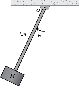
We first draw the free-body diagram where the forces acting on the pendulum are its weight and the reaction at the rotational joint. We also include a moment due to the friction in the joint (and the rotary potentiometer). The simplest approach to modeling assumes the mass of the bar is negligible and that the entire mass of the pendulum is concentrated at the center of the end weight.
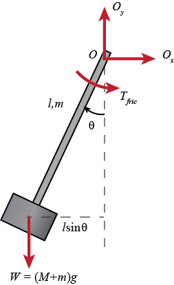 |
- The equation of motion of the pendulum can then be derived by summing the moments.
- We will choose to sum the moments about the attachment point $O$ since that point is the point being rotated about and since the reaction force does not impart a moment about that point.
We can then write:
$$ \sum{M} = (M+m)glsin(\theta) - T_{fric} = I_O\ddot\theta$$
Assuming that the mass of the pendulum is concentrated at its end mass, the mass moment of inertia is $I_O \approx (M+m)l^2$. A more accurate approach would be to consider the rod and end mass explicitly. In that case, the weight of the system could be considered to be located at the system's mass center $l_G = (Ml+0.5ml))/(M+m)$. In that case, the mass moment of inertia is $I_O = ml^2/3 + Ml^2$. Depending on the parameters of your particular pendulum, you can assess if this added fidelity is necessary.
We will also initially assume a viscous model of friction, that is, $T_{Fric} = -b\dot{\theta}$ where $b$ is a constant. Such a model is nice because it is linear. We will assess the appropriateness of this model later. Sometimes the frictional moment is not linearly proportional to the angular velocity. Sometimes, the stiction in the joint is significant enough that it must be modeled too.
Taking into account the above assumptions, our equation of motion becomes the following.
$$ -(M+m)gl_G\sin\theta - b\dot{\theta} = I_O\ddot{\theta} $$
We will use the same parameters of this pendulum.
This is a simple pendulum that consists of:
- a rod of length $l = 0.43\ \mbox{m}$ and mass $m = 0.095\ \mbox{kg}$
- an end mass of $0.380\ \mbox{kg}$.
Assuming that the mass of the pendulum is concentrated at its end mass, the mass moment of inertia is $I_O \approx (M+m)l^2$. A more accurate approach would be to consider the rod and end mass explicitly. In that case, the weight of the system could be considered to be located at the system's mass center $l_G = (Ml+0.5ml))/(M+m)$. In that case, the mass moment of inertia is $I_O = ml^2/3 + Ml^2$. Depending on the parameters of your particular pendulum, you can assess if this added fidelity is necessary.
Therefore, the difference between $l = 0.43\ \mbox{m}$ and $l_G = 0.39\ \mbox{m}$ is significant enough to include.
The difference between $I_O \approx (M+m)l^2 = 0.088\ \mbox{kg-m}^2$ and $I_O = ml^2/3 + Ml^2 = 0.076\ \mbox{kg-m}^2$ is also significant enough to include.
After model identification the following parameters are identified:
$$ I_O = 0.079\ \mbox{kg-m}^2 $$ $$ b = 0.003\ \mbox{N-m-s}^2 $$
Recalling the model we derived from first principles earlier.
$$ I_O\ddot{\theta} + b\dot{\theta} + (M+m)gl_G\sin\theta = 0 $$
The final equation is:
$$ 0.079\ddot{\theta} + 0.003\dot{\theta} + 1.82\sin\theta = 0 $$We can write this as:
$$\dot{x_1}= x_2$$ $$\dot{x_2}=\frac{1}{0.079}\big ( -1.82\sin x_1 -0.003 x_2 \big)$$
We now create our pendulum with specific initial conditions
pendulum = Pendulum( theta_0 = 0.423, theta_dot_0 = 0, params=PendulumParameters())
And finally we define the simulation parameters and run the simulation
t0, tf, dt = 0, 15, 0.01 # time

angle = []
time = np.arange(t0, tf, dt)
for t in time:
    pendulum.step(dt, u=0.0)
    angle.append(pendulum.sense_theta_deg())
Let's plot the results:
fig, ax = plt.subplots(1, 1, figsize=(15, 5))
plt.plot(time, angle, linewidth=3)
plt.grid()
plt.yticks(np.arange(-30, 30, step=5))  # Set label locations.
plt.ylabel('angle (deg)')
plt.xlabel('time (s)');

As expected the pendulum oscillates, with decreasing amplitude which depends on the damping coefficient (try different values of the viscous friction coefficient $b$ in the class parameter to see how it affects the response).
We can also verify what happens when we apply an esternal torque $u$
params = PendulumParameters()
params.b = 2
pendulum = Pendulum( theta_0 = np.radians(10), theta_dot_0 = 0, params=params)
t0, tf, dt = 0, 15, 0.01 # time

angle = []
time = np.arange(t0, tf, dt)
for t in time:
    pendulum.step(dt, u=0.31)
    angle.append(pendulum.sense_theta_deg())

fig, ax = plt.subplots(1, 1, figsize=(15, 5))
plt.plot(time, angle, linewidth=3)
plt.grid()
plt.yticks(np.arange(-10, 30, step=5))  # Set label locations.
plt.ylabel('angle (deg)')
plt.xlabel('time (s)');

Let's now animate the pendulum so that we can get a better intuition of how it behaves.
The PendulumDrawer class does the animation manually, drawing each single frame explicitely. Using this method results in quite slow rendering performance. We will use the FuncAnimation to solve this issue. For now, let's see how the PendulumDrawer class could be defined.
pendulum_drawer = PendulumDrawer(pendulum)
fig, ax = plt.subplots(1,1)
pendulum_drawer.draw(ax)
plt.title('theta: {:.1f} deg'.format(pendulum_drawer._pendulum.sense_theta_deg()))
plt.axis('equal');

If we used the PendulumDrawer class our rendering will be very slow.
Let's now leverage matplotlib functionalities directly to have a better animation. This is done through the class AnimatePendulum.
And now we can put everything together and animate our pendulum!
t0, tf, dt = 0, 10, 1./30 # time
ap = AnimatePendulum(Pendulum(theta_0=np.radians(10), theta_dot_0=0, params=PendulumParameters()), t0, tf, dt)
ap.simulate(u=0.31);
ap.start_animation()

class DCMotorParams():
    def __init__(self, J=0.01, b=0.1, K=0.01, R=1, L=0.5):
            #     (J)     moment of inertia of the rotor     0.01 kg.m^2
            #     (b)     motor viscous friction constant    0.1 N.m.s
            #     (Ke)    electromotive force constant       0.01 V/rad/sec
            #     (Kt)    motor torque constant              0.01 N.m/Amp
            #     (R)     electric resistance                1 Ohm
            #     (L)     electric inductance                0.5 H
            #      Note that in SI units, Ke = Kt = K
        self.J = J
        self.b = b
        self.K = K
        self.R = R
        self.L = L

class DCMotor():
    def __init__(self, x0, params):
        self._params  = params

        self._x0 = x0
        self._x = x0
        self._J_load = 0
        self.update_motor_matrix()

    def update_motor_matrix(self):
        # state variables are: rotation speed (w, or theta_dot) and current (i)
        self._A = np.array([[-self._params.b/(self._params.J+self._J_load),  self._params.K/(self._params.J+self._J_load)],
                            [-self._params.K/self._params.L,  -self._params.R/self._params.L]])
        self._B = np.array([[0],[1/self._params.L]])
        self._C = np.array([1,   0])
        self._D = 0;

    def reset(self):
        self._x = self._x0

    def set_load(self, J_load):
        self._params.J += J_load
        self.update_motor_matrix()

    def step(self, dt, u):
        self._x = self._x + dt*(self._A@self._x + self._B*u)

    def measure_speed(self):
        self._y = self._C@self._x
        return self._y
motor = DCMotor(np.array([[0], [0]]), DCMotorParams())
y = []
u = 1

time_vector = np.arange(0, 10, 0.01)
for t in time_vector:
    motor.step(0.01, u)
    y.append(motor.measure_speed())
fig = plt.figure(figsize=(10,5))

plt.plot(time_vector, y)
plt.xlabel('time (s)')
plt.ylabel('speed (w, rad/s)')

motor.reset()
motor.set_load(0.1)
y = []
u = 1

time_vector = np.arange(0, 10, 0.01)
for t in time_vector:
    motor.step(0.01, u)
    y.append(motor.measure_speed())
fig = plt.figure(figsize=(10,5))

plt.plot(time_vector, y)
plt.xlabel('time (s)')
plt.ylabel('speed (w, rad/s)')

We modify the usual definition of the motor (see above), adding one state to explicit the rotor position.
We also define a wrapping function to make sure the rotor position stays within -pi and pi.
motor = DCMotor(x0=np.array([[0], [0], [0]]), params=DCMotorParams())
y = np.array([[0],[0]]) # initialise to 0. This is only here to have the correct size. Alternative: y = np.empty((2,1))

u = 1

time_vector = np.arange(0, 10, 0.01)
for t in time_vector:
    motor.step(0.01, u)
    y = np.append(y, motor.measure(), axis=1)

# remove the first item which was there only to have the correct size
y = np.delete(y, 0, axis=1)

position = y[0,:]
velocity = y[1,:]
fig, axs = plt.subplots(2, 1, figsize=(10,5))

axs[0].plot(time_vector, velocity)
axs[0].set_xlabel('time (s)')
axs[0].set_ylabel('speed (w, rad/s)')

axs[1].plot(time_vector, position)
axs[1].set_xlabel('time (s)')
axs[1].set_ylabel('position (rad)');

Or if we want to express it as a transfer function: $$ P(s) = \frac{\dot\Theta(s)}{V(s)} = \frac{K}{(Js+b)(Ls+R) + K^2} $$
and if we want to measure the position
$$ \tilde{P}(s) = \frac{\Theta(s)}{V(s)} = \frac{K}{s(Js+b)(Ls+R) + K^2} $$We can now control the position of the motor
motor = DCMotor(x0=np.array([[0], [0], [0]]), params=DCMotorParams())
Kp = 10
Kd = 3
Ki = .1

y_history = np.array([[0],[0]]) # initialise to 0. This is only here to have the correct size. Alternative: y = np.empty((2,1))
error_history = np.array([[0]])

ref_position = np.radians(1) # position reference
time_vector = np.arange(0, 10, 0.01)

error_old = 0
error_dot = 0
error_I  = 0
for t in time_vector:
    y = motor.measure()
    position, velocity = y[0], y[1]
    error = ref_position - position
    error_dot = (error - error_old)/0.01
    error_I   += error*0.01
    error_old = error
    # controller
    u = Kp*error + Kd*error_dot + Ki*error_I
    motor.step(0.01, u)

    # save the last measurements
    y_history = np.append(y_history, y, axis=1)
    error_history = np.append(error_history, [error], axis=1)


# remove the first item which was there only to have the correct size
y_history = np.delete(y_history, 0, axis=1)
error_history = np.delete(error_history, 0, axis=1)

position = y_history[0,:]
velocity = y_history[1,:]
error = error_history[0,:]

print('Reference (rad)/(deg): {:.5f}/{:.2f}'.format(np.radians(ref_position), ref_position))
fig, axs = plt.subplots(3, 1, figsize=(10,5))

axs[0].plot(time_vector, velocity)
axs[0].set_xlabel('time (s)')
axs[0].set_ylabel('speed (w, rad/s)')


axs[1].plot(time_vector, position)
axs[1].plot(time_vector, ref_position*np.ones(position.shape))
axs[1].set_xlabel('time (s)')
axs[1].set_ylabel('position (rad)');

axs[2].plot(time_vector, np.degrees(error))
axs[2].set_xlabel('time (s)')
axs[2].set_ylabel('error (deg)');

And now we can define it as a class.
To be honest, this class will do more than simply controlling the motor, but will do for now.
p_params = PendulumParameters()
p_params.b = 0.2

m_params = DCMotorParams()
pendulum = Pendulum(theta_0=np.radians(0), theta_dot_0=0, params=p_params)
motor = DCMotor(x0=np.array([[0], [0], [0]]), params=m_params)
motor_controller = MotorController(Kp=1000, Kd=500, Ki=1000, motor=motor)

# connect the motor to the pendulum
motor.connect_to(pendulum)

t0, tf, dt = 0, 20, 0.01
time_vector = np.arange(t0, tf, dt)

ref_position_rad=np.radians(5)
angle = []
for t in time_vector:
    motor_controller.run(dt,
                         ref_position_rad=ref_position_rad,
                         y = np.array([[np.radians(pendulum.sense_theta_deg())], [pendulum.speed()]]))
    T = motor_controller.motor.get_motor_torque()
    pendulum.step(dt, u=T)
    angle.append(pendulum.sense_theta_deg())


position, velocity, error, torque = motor_controller.get_results()

print('Reference position: {:.4f} rad/{:.1f} deg'.format(ref_position_rad, np.degrees(ref_position_rad)))
print('Pendulum position (tf): {:.4f} rad/{:.1f} deg'.format(np.radians(angle[-1]), angle[-1]))
fig, axs = plt.subplots(5, 1, figsize=(10,10))

axs[0].plot(time_vector, velocity)
axs[0].set_xlabel('time (s)')
axs[0].set_ylabel('motor speed (w, rad/s)')

axs[1].plot(time_vector, position)
axs[1].plot(time_vector, ref_position_rad*np.ones(position.shape))
axs[1].set_xlabel('time (s)')
axs[1].set_ylabel('motor position (rad)');

axs[2].plot(time_vector, np.degrees(error))
axs[2].set_xlabel('time (s)')
axs[2].set_ylabel('motor error (deg)');

axs[3].plot(time_vector, torque)
axs[3].set_xlabel('time (s)')
axs[3].set_ylabel('torque (N.m)');

axs[4].plot(time_vector, angle)
axs[4].plot(time_vector, np.degrees(ref_position_rad)*np.ones(position.shape))
axs[4].set_xlabel('time (s)')
axs[4].set_ylabel('pendulum position (deg)');
axs[4].set_ylim(0, 20)

plt.tight_layout()

p_params = PendulumParameters()
p_params.b = 0.2
m_params = DCMotorParams()
pendulum = Pendulum(theta_0=np.radians(20), theta_dot_0=0, params=p_params)
motor = DCMotor(x0=np.array([[0], [0], [0]]), params=m_params)
controller = MotorController(Kp=1000, Kd=500, Ki=1000, motor=motor)


t0, tf, dt = 0, 10, 1./30 # time
ap = AnimateControlledPendulum(pendulum, motor, controller, t0, tf, dt)
ap.simulate(angle_ref=10, controller_flag=True);
ap.start_animation()