Please fill up the questionnaire at: https://esami.unipi.it
Install Anaconda: Anaconda Download Page
Refer to the Anaconda documentation for more information here
Open a terminal window:
- Windows: From the Start menu, search for and open “Anaconda Prompt”
- MacOS/Linux: Click the terminal icon.
Once in a terminal,
- create an environment:
conda create --name env-automatic-control python=3.9 - activate it:
conda activate env-automatic-control
- create an environment:
Install everything that is needed
Jupyter notebook:
conda install -c conda-forge notebookStandard engineering libraries:
python -m pip install matplotlib numpy pandasconda install numpy scipy matplotlib# if not yet installedconda install -c conda-forge controlconda install -c anaconda sympy
You are set up!
Going back to work (opening your Jupyter notebooks)
Open a terminal window:
- Windows: From the Start menu, search for and open “Anaconda Prompt”
- MacOS/Linux: Click the terminal icon.
Move to yur project folder (e.g.
cd /Users/<USERNAME>/MyProject/)
(if you need to find out how to find your folder path in Windows read below: "Note: To find out where is your folder in Windows")Activate your conda environment:
conda activate env-automatic-controlRun:
jupyter notebook
A new tab in your browser should open up automatically showing the jupyter home folder (your current folder).
If it does not open, open your favourite brower and type: localhost:8888 in the browser address bar.
Sometime jupyter requires a token - this is automatically created when jupyter is started. Look back to your terminal window right after the command jupyter notebook there should be a line similar to:
To access the notebook, open this file in a browser:
    file:///Users/<YOUR_USERNAME>/Library/Jupyter/runtime/nbserver-73848-open.html
Or copy and paste one of these URLs:
    http://localhost:8888/?token=66781622f3ed474ccf1f0f61e5708b035acfcf4e41cc7c8a
 or http://127.0.0.1:8888/?token=66781622f3ed474ccf1f0f61e5708b035acfcf4e41cc7c8a
Copy and paste one of the last two addresses in your browser to start your jupyter session.
You are ready to start coding!
Note: To find out where is your folder in Windows:
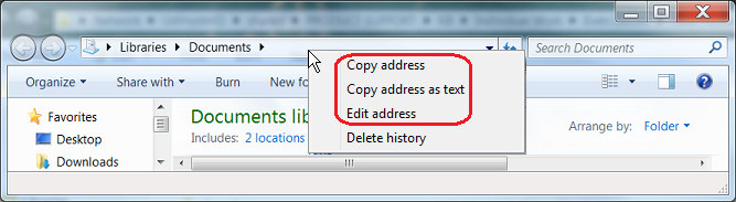
- Open Windows Explorer and go inside the folder you need
- Right click on the address path and right-click
- Select "copy address as text" (see picture below)
- Go back to your Anaconda prompt and paste it (remember to type
cdfirst!)
 |
References
- Systems and control systems
Three problems:
- system identification problem
- simulation problem
- control Problem
Why do we need feedback control
Transfer Functions
- Laplace domain representation of a system
Definition:Transfer function is the Laplace transform of the impulse response of a linear, time-invariant system with a single input and single output when you set the initial conditions to zero.
- State space vs Transfer functions
- Laplace Transform
The Laplace transform is important because it is a tool for solving differential equations: it transforms linear differential equations into algebraic equations, and convolution into multiplication!
- Derivatives and integrals become algebric operations
From a system perspective, the Transfer function expresses the relation between the Laplace Transform of the input and that of the output:
$$ Y(s)=\mathbf{c}^T(s\mathbf{I}-\mathbf{A})^{-1} \mathbf{b} U(s) $$
Properties of the Laplace Transform (relationships between time and frequency)
- $\frac{df}{dt}(t) \rightarrow sF(s)$
- $af(t)$ + $bg(t) \rightarrow aF(s)+bG(s)$
Laplace transforms of known functions:
- $\delta(t) \rightarrow 1$
- $1(t) \rightarrow \frac{1}{s}$
- $e^{-at} \rightarrow \frac{1}{s+a}$
- ...
- System $G(s)$ is asymptotically stable if all its poles have $Re<0$
- System $G(s)$ is stable if all its poles have G(s) $Re \le 0$ and if those with $Re=0$ have multiplicity one.
- System $G(s)$ is unstable if it has at least one pole with $Re>0$ or with $Re=0$ and multiplicity $\ge 2$.
- BIBO stability:
- A system is BIBO stable (Bounded Input, Bounded Output) if for each limited input, there is a limited output
- For linear systems: BIBO stability if and only if poles of the transfer functions have $Re<0$
- Stability of a system in a state space representation
- Controllability (Reachability)
- Observability
System Response
- Dominant pole approximation
First-order and second-order systems
- First-order systems: step response and performance
- time constant ($\tau$) - Characterises completely the response of a first order system
settling time: $t_s = -\tau ln(0.05)$ (time to get to 95% of steady state)
Second order systems: step response and performance
- More parameters to define performance: max overshoot, time of max overshoot, settling time, oscillation period
Frequency response
- Assuming that the system is asymptotically stable,
- If we input a sinusoid $Asin(\omega t)$
- The output of the system converges $y(t)=A|G(j\omega)|sin(\omega t + \angle G(j\omega) ) $
- $G(j\omega)$ is the frequency response
- If we know magnitude and phase of $G(j\omega)$ (for varying $\omega$) then we know how the system behaves for all sinusoidal inputs with different driving frequencies.
Bode plots
Frequency Response and Bode Plots
- analysing the gain and the phase shift across the full frequency spectrum
- gain diagram and phase diagram
Leverages the properties of transfer functions and of logarithms:
- The transfer function of linear systems are polynomial fractions in $s$
- It is always possible to factor polynomials in terms of their roots (zeros and poles)
- Each polynomial is the product of first-order or second-order (potentially with multiplicity $>$ 1)
- To build the frequency response of the system is useful to have simple rules to represent each term
- The logarithm of a product is equal to a sum of logarithms
- remember to convert gain to dB: $|G(j\omega)|_{dB}=20log_{10}|G(j\omega)|$
Sketching Bode Plots
- Given a transfer function $G(s)$ we can obtain the (steady state) frequency response setting $s=j\omega \rightarrow G(j\omega)$
- $G(j\omega) = \text{real} + \text{imag}j $
- Gain: $\sqrt{\text{real}^2 + \text{img}^2} = |G(j\omega)|$
- Phase: $atan2(\text{img}, \text{real}) = arg(G(j\omega)) = \angle G(j\omega)$
- Our building blocks:
- constant gain
- integrator
- simple pole
- complex poles
- specular behaviour for the zeros (properties of the logarithms)
- Transform the trasnfer function to the Bode form before drawing the Bode plots!
Final value theorem and steady state error
- Meaning of final value
- Theorem: for an asymptotically stable LTI system: $ \lim\limits_{t \rightarrow \infty} x(t) = \lim\limits_{s \rightarrow 0} sX(s)$
- System type: number of poles at the origin
- Analysis of the final value for different system types and different inputs
- For a feedback system: the final value of the error is a much better indicator of the performance of our controller
Diving deeper into the feedback loop
- Included load disturbances and measurement noise in the feedback loop
- Sensitivity function (feedback and disturbances / low frequency specifications)
- Complementary sensitivity function (feedback and measurements / high frequency specifications)
- Design requirements on the loop gain function $|R(s)G(s)|$