- Calculate the Laplace Transform $X(s)$ of the signal $x(t)$:
Let's verify it with Sympy
import matplotlib.pyplot as plt # import matplotlib - it will be useful later.
import sympy # import sympy
t, s = sympy.symbols('t, s')
f1 = 4*t*sympy.exp(-2*t)
f2 = - 3*sympy.cos(5*t)*sympy.exp(-2*t)
print('{} {}'.format(f1, f2))
F1 = sympy.laplace_transform(f1, t, s, noconds=True)
F2 = sympy.laplace_transform(f2, t, s, noconds=True)
print('{} {}'.format(F1, F2))
- Calculate the Inverse Laplace Transform $g(t)$ of the transfer function $G(s)$:
F1 = 2
F2 = 3/(2*s**3+3*s**2+s)
f1 = sympy.inverse_laplace_transform(F1, s, t)
f2 = sympy.inverse_laplace_transform(F2, s, t)
print('{} + {}'.format(f1, f2))
f3 = sympy.inverse_laplace_transform(F1+F2, s, t)
print('{}'.format(f3))
- Write the transfer function to a step input of a second order system characterised by:
- Static gain $G(0)=5$
- Damping ratio $\xi=0.5$
- Settling time $t_s=3 s$
- No zeros
We would like a system with form: $$ \frac{K}{s^2+2\xi\omega_ns+\omega_n^2} $$
we also know that:
$$ t_s \approx -\frac{1}{\xi\omega_n}ln(0.05)\;\; s $$from which:
$$ \omega_n = -\frac{1}{3\cdot0.5}ln(0.05) = 2 \;\; rad/s $$which means:
$$ \frac{K}{s^2+2s+4} $$since we want $G(0)=5 \rightarrow K=20$
$$ \frac{20}{s^2+2s+4} $$- Plot the qualitative behaviour of the step response of the system:
Let's re-write the transfer function slightly:
$$ G(s)=\frac{20\cdot0.1(30+s)(s^2+10s+160)}{2(s+\frac{10}{2})0.1(s+\frac{5}{0.1})(s^2+2s+400)} $$The poles are:
$$ s = -5, -50, -1.+19.97498436j, -1.-19.97498436j $$and the zeros are:
$$ s = -30, -5.+11.61895004j, -5.-11.61895004j $$The system is asymptotically stable, we can use the dominant poles approximation:
$$ G(s)=\frac{20\cdot0.1\cdot30\cdot160}{2\cdot5\cdot0.1\cdot50(s^2+2s+400)} = \frac{192}{(s^2+2s+400)} $$The response to a step input can be obtained as:
$$ Y(s) = G(s)\frac{1}{s} = \frac{192}{(s^2+2s+400)}\frac{1}{s} $$And, using partial fraction decomposition:
$$ Y(s) = \frac{K}{s} + \frac{A}{s-p_1} + \frac{A^*}{s-p_1^*} $$Where
$$ K = \frac{192}{(s^2+2s+400)} \bigg |_{s=0} = \frac{192}{400} = 0.48 $$And for the pole $p_1=−1.+19.97498436𝑗$
We know that when we have complex conjugate poles - see notebook 03_Transfer_function:
where:
$$ A = (s-p_1)\frac{192}{s(s-p_1)(s-p_1^*)} \bigg |_{s=-1+20j} = \frac{192}{s(s-p_1^*)} \bigg |_{s=-1+20j} = \frac{192}{(-1+20j)( 40j)} = -0.24+0.012j $$abs(-0.24+0.012)
abs(192/(40j*(-1+20j)))
import numpy as np
np.sqrt(399)
and the response is
$$ y(t) = K + Ae^{p_1}t + A^*e^{p_1^*}t = K + 2|A|e^{\sigma t}cos(\omega t + \angle{A}) $$where $p_1=\sigma+\omega t$ and $A=|A|e^{j\angle{A}}$
We can check that the inverse laplace of the system transfer function using Sympy:
def evaluate(f, times):
    res = []
    for time in times:
        res.append(f.evalf(subs={t:time}).n(chop=1e-5))
    return res
def L(f):
    return sympy.laplace_transform(f, t, s, noconds=True)
def invL(F):
    return sympy.inverse_laplace_transform(F, s, t)
t, s = sympy.symbols('t, s')
F = 192/(s**2+2*s+400)
invL(F)
Where:
import numpy as np
import cmath
np.sqrt(399)
And now we can plot it to verify the step response:
time = np.linspace(0, 7, 1000)
y = 0.48 + 2*0.23*np.exp(-time)
plt.plot(time, y)
plt.xlabel('time');

Finally, let's compare the result we got with what Sympy calculates
fig, ax = plt.subplots(1,1,figsize=(8,5))

time = np.linspace(0,7,1000)

ax.plot(time, evaluate(invL(F*1/s), time), linewidth=3)
ax.plot(time, y, 'g')

ax.set_title(f'y(end)={y[-1]}');

Let's look at the response more closely:
plt.plot(time[:100], y[:100])

We can also use the Python Control Library to verify our dominant pole approximation
import control
import matplotlib.pyplot as plt
s = control.TransferFunction.s
G = (20*(3+0.1*s)*(s**2+10*s+160))/((2*s+10)*(0.1*s+5)*(s**2 + 2*s + 400))
G_approx = 192/(s**2 + 2*s + 400)
T, yout = control.step_response(G, T=np.linspace(0, 7, 1000));
Tap, youtap = control.step_response(G_approx, T=np.linspace(0, 7, 1000));

plt.plot(T, yout, 'b', label='original')
plt.plot(Tap, youtap, 'r', label='approx d.p.')
plt.legend()
plt.grid()

- For the system $G(s)$ defined above, calculate:
- Its steady state value $y_\infty$ to a step input (when $t \rightarrow \infty$)
- Its settling time $t_s$
- If the system oscillates, calculate the period $T_\omega$ of the oscillation
- $y(t\rightarrow\infty) = 0.48$
- $t_s \approx -\frac{1}{\xi\omega_n}ln(0.05) \approx 3$
given that:
- $\omega_n=\sqrt{399}\approx20$
- $2\xi\omega_n=2 \rightarrow 20 \xi =1 \rightarrow \xi = 0.05$
And finally:
- $T_{P} = \frac{2\pi}{w_n\sqrt{1-\xi^2}} = 0.314s$
xi = 0.05
wn = 20
t_s = -1/(xi*wn)*np.log(0.05)
print('t_s = {}'.format(t_s))

Tp = 2*3.14/(wn*np.sqrt(1-xi**2))

print('T_p = {}'.format(Tp))
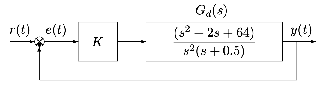
The characteristic equation of the feedback system is:
$$ 1+K\frac{s^2+2s+64}{s^2(s+0.5)} = 0 \rightarrow s^2(s+0.5)+K(s^2+2s+64) = 0 \rightarrow s^3 + (0.5+K)s^2 + 2Ks+64K=0 $$The Routh table is:
| $3$ | $1$ | $2K$ |
| $2$ | $0.5+K$ | $64K$ |
| $1$ | $(0.5+K)2K-64K$ | $0$ |
| $0$ | $64K$ |
from which it is possible to find the following constraints on $K$:
$$ 0.5 + K > 0, \hspace{0.5cm} 2K^2 +1K-64K > 0, \hspace{0.5cm}K>0 $$And the system is asymptotically stable for $K>31.5$
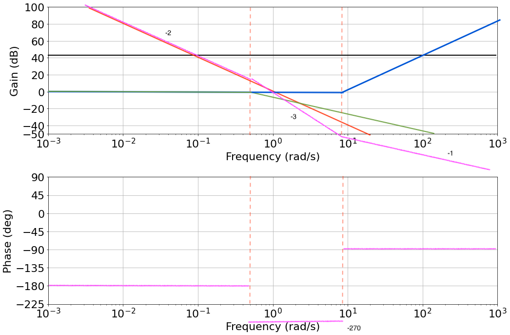
$K_{dB}=20\log(64/0.5) \approx 42 dB$
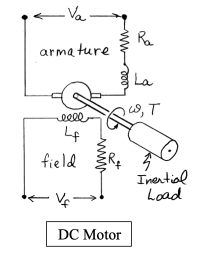
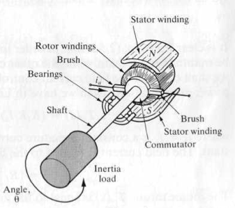
DC Motor Transfer Functions
The figures below represents a DC motor attached to an inertial load.
 |
 |
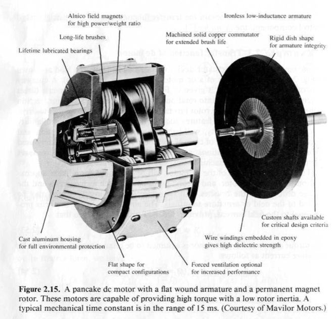 |
The input voltage can be applied to either the field or the armature terminals. The voltages applied to the field and armature sides of the motor are represented by $V_f$ and $V_a$.
The resistances and inductances of the field and armature sides of the motor are represented by $R_f$ , $L_f$, $R_a$, and $L_a$. The torque generated by the motor can be assumed to be related linarly to $i_f$ and $i_a$, the currents in the field and armature sides of the motor, as follows:
$$ T_m = K i_f i_a \;\;\;\;(1) $$From the equation above, clearly to retain the linearity, one current must be kept constant, while the other becomes the input current.
This makes it possible to have field-current or armature-current controlled motors. We will focus on the field-current motor for our analysis.
This means that in a field-current controlled motor, the armature current is kept constant, while the field current $i_a$ is controlled through the field voltage $V_f$.
$$ T_m = K i_f i_a = K_m i_f \;\;\;\;(2) $$where $K_m$ is defined as the motor constant. The motor torque increases linearly with the field current.
1. Write the Transfer Function from the input current to the resulting torque of the previous equation
For the field side of the motor the voltage/current relationship is $$ V_f =V_R +V_L = R_f i_f +L_f (di_f dt) \;\;\;\;(3) $$
2. Write the Transfer Function from the input voltage to the resulting current
Vf = RfI+LsI
I = Vf/Lf/(Rf/Lf+s)
$$ \frac{I_f(s)}{V_f(s)} = \frac{\frac{1}{L_f}}{s+\frac{R_f}{L_f}} \;\;\;\;(4) $$3. Write the Transfer Function from the input voltage to the resulting motor torque
$$ \frac{T_m(s)}{V_f(s)} = \frac{\frac{K_m}{L_f}}{s+\frac{R_f}{L_f}} \;\;\;\;(5) $$4. Discuss how the motor torque behaves with respect to different input signals (e.g., step input in field voltage, etc.)
This is a first-order system (type 0), and a step input in field voltage $V_f$ results in an exponential rise in the motor torque.
We can now add load to the motor and verify how its behaviour changes.
The motor torque $T_m(s)$ is equal to the torque delivered to the load, and this relation can be expressed as:
$$ T_m(s) = T_L(s) + T_d(s) \;\;\;\;(6) $$where $T_L(s)$, and $T_d(s)$ is the disturbance torque (e.g., external forces acting on the load).
We can calculate the rotational motion of the inertial load summing moments (see Figures above):
$$ \sum{M} = T_L - f\omega = J \dot{\omega} \;\;\;\;(7) $$where $f$ is due to friction, and $J$ is the load inertia.
5. Write the Laplace transform of the load torque $T_L(s)$ using using equation (7) above
6. Given that the relationship between position and angular velocity $\omega$, refine the equation you have just calculated to explicit the rotor position $\theta$ (hint: $\dot\theta = \omega$)
where $\Omega(s) = \mathcal{L}(\omega(t))$
7. Put together equations (2,4,6) and calculate the transfer function of the motor-load combination
$$ \frac{\theta(s)}{V_f(s)} = \frac{K_m}{s(Js+f)(L_fs+R_f)} = \frac{\frac{K_m}{JL_f}}{s(s+\frac{f}{J})(s+\frac{R_f}{L_f})}. \;\;\;\;(8) $$8. Discuss the resuting system (order, dominant pole approximations, what happens when parameters change, select specific values for the parameters and draw its step response.)
$$ \frac{\theta(s)}{V_f(s)} = \frac{\frac{K_m}{JL_f}}{s(s+\frac{f}{J})(s+\frac{R_f}{L_f})} = \frac{\frac{K_m}{fR_f}}{s(\tau_f s+1)(\tau_L s+1)} $$where $\tau_f=\frac{L_f}{R_f}$ and $\tau_L=\frac{J}{f}$.
When $\tau_L > \tau_f$, the field time constant $\tau_f$ can be neglected.
Let's choose the following values:
- (J) moment of inertia of the rotor 0.01 kg.m^2
- (f) motor viscous friction constant 0.1 N.m.s
- (Ke) electromotive force constant 0.01 V/rad/sec
- (Kt) motor torque constant 0.01 N.m/Amp
- (R) electric resistance 1 Ohm
- (L) electric inductance 0.5 H
_Note that in SI units, $K_e = K_t = K$_
s = control.TransferFunction.s
G_motor = 0.1/(s*(0.5*s+1)*(0.1*s+1))
T, yout = control.step_response(G_motor, T=np.linspace(0, 7, 1000));

plt.plot(T, yout, 'b', label='dc-motor-step-response')
plt.legend()
plt.xlabel('time')
plt.grid()

9. Draw a block diagram of the field controlled DC motor from the field voltage to the position output using all the relevant equations calculated so far. Make sure you include the disturbance $T_d(s)$ as per equation (6).
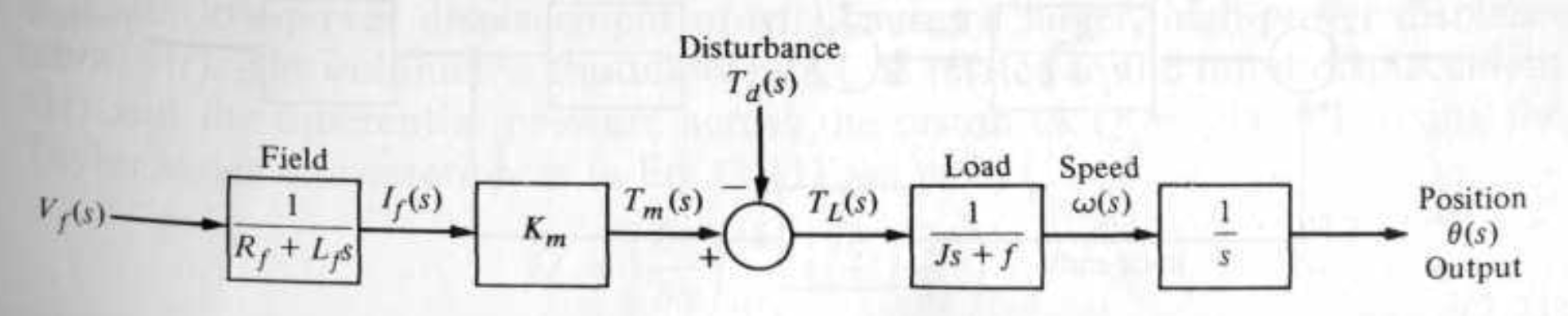 |