import numpy as np
import matplotlib.pyplot as plt
import control
- The PID controller is the most common form of feedback.
- Standard tool when process control emerged in the 1940s.
In process control today, more than 95% of the control loops are of PID type
- Most loops are PI control.
PID control is often combined with logic, sequential functions, selectors, and simple function blocks to build more complicated automation systems
- Sophisticated control strategies, such as model predictive control, are also organized hierarchically.
- PID control is used at the lowest level: high level controller gives the setpoints (the reference variables) to the controllers at the lower level.
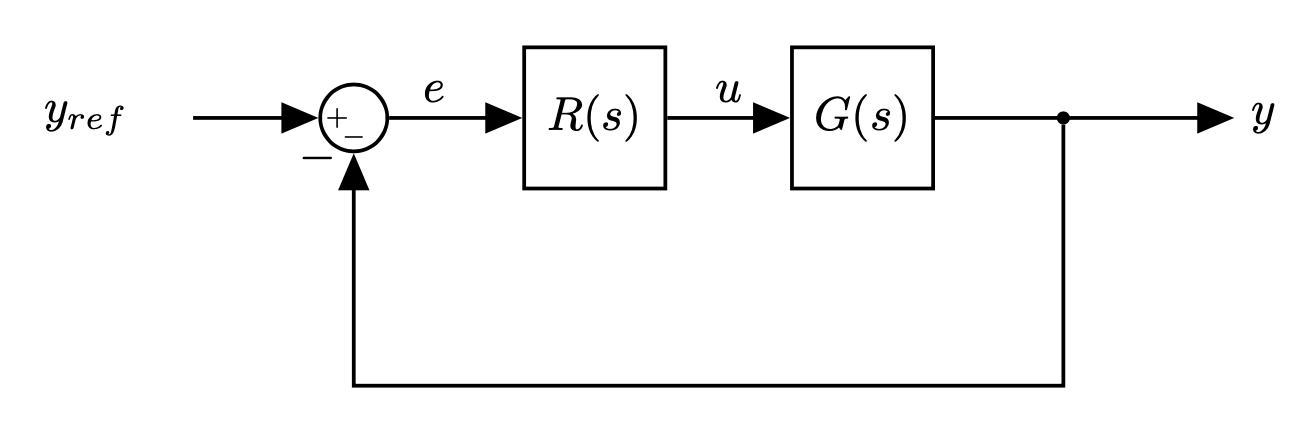 |
- A common way to design a control system is to use PID control.
PID = Proportional-Integral-Derivative
- Describes how the error term is treated before being sum and sent into the plant
It is a simple and effective controller in a wide range of applications
- Majority of controllers in industrial applications are PIDs
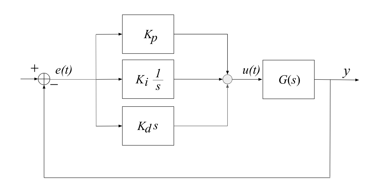
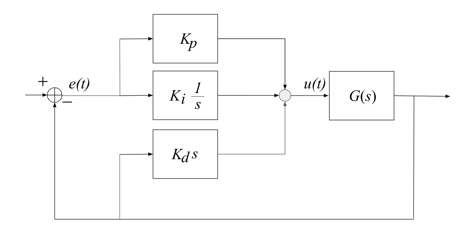
The general structure of a PID controller is:
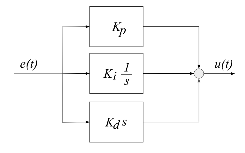 |
- The three gains $K_p, K_i, K_d$ are adjustable and can be tuned to the specific application
- Varying $K_p, K_i, K_d$ means adjusting how sensitive the system is across the three paths
The "textbook" version of the PID algorithm is:
$$ u(t) = K\Big(e(t) + \frac{1}{T_i}\int_0^t e(\tau)d\tau + T_d\frac{de(t)}{dt} \Big) $$Will consider each in turn, using an example transfer function
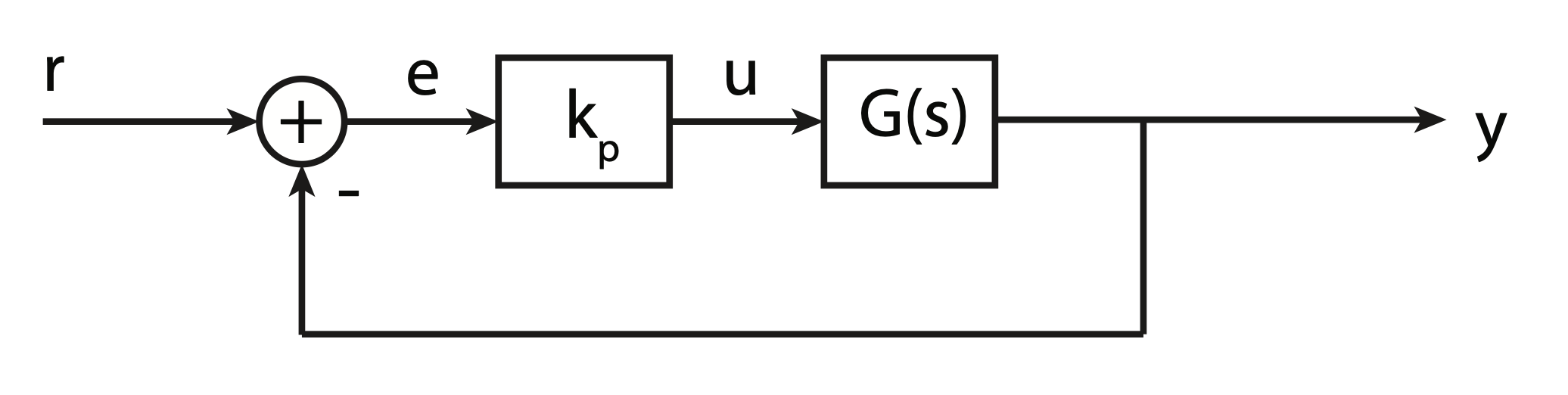
$$ G(s) = \frac{A}{s^2+a_1s+a_2} $$Let's consider our system and its characteristic equation:
$$ 1 + K_p G(s) = 0 $$
$$ 1 + K_p \frac{A}{s^2+a_1s+a_2} = 0 $$
$$ \Rightarrow s^2+a_1s+a_2 + K_pA = 0 $$
Since we know:
$$ s^2+2\zeta\omega_n s+ \omega_n^2 = 0 $$$$ s_{1,2} = -\zeta\omega_n \pm \omega_n\sqrt{(1-\zeta^2)}j $$The resulting natural frequency is:
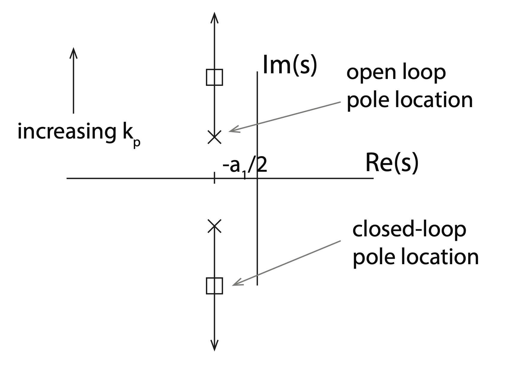
$$ w_n = \sqrt{a_2+K_pA} $$
- Increasing $K_p$ increases the natural frequency,
- Note that the dumping ratio is reduced (we do not change $a_1$).
If we plot the position of the poles in the Root Locus:
 |
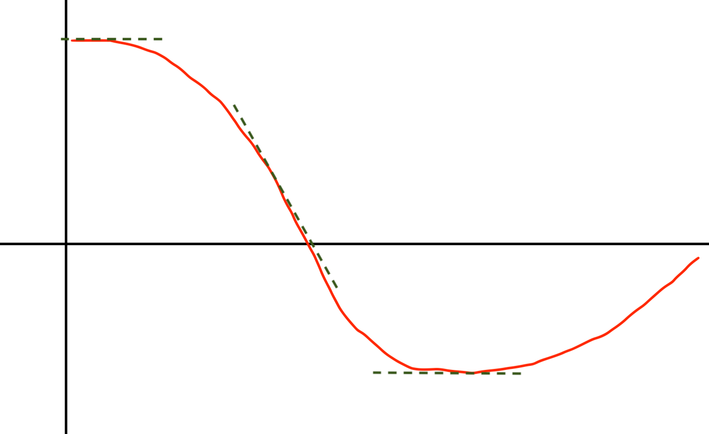
Proportial error and output:
 |
- Output is the error scaled by the gain $K_p$
- When error is large, output is large
- When error is small, output is small
To add damping to a system, it is often useful to add a derivative term to the control,
$$ u(t) = K_p e(t) + K_d\dot{e}(t) $$or
$$ U(s) = K_p E(s) + K_d sE(s) = (K_p+K_ds)E(s) = K(s) E(s) $$And the characteristic equation is:
$$ 0 = 1+K(s)G(s) $$$$ 1 + \frac{(K_p + K_ds) A}{s^2+a_1s+a_2} $$$$ 0 = s^2 + (a_1+K_dA)s + (a_2 + K_p) $$- In this example, increasing K_d increases the damping ratio without changing the natural frequency.
- For other $G(s)$ the result might differ!
When we keep $K_p$ fixed, and vary $K_d$ the Root Locus changes:
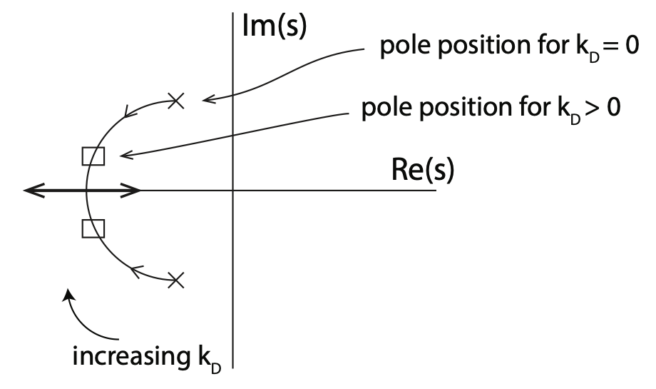 |
- In the derivative path is the rate of change of the error that contributes to the output of the controller
- The faster the change the larger the output
 |
Especially if the plant is a type 0 system, we may want to add integrator to controller to drive steady-state error to zero:
$$ U(s) = (K_p + \frac{K_I}{s} + K_d s) E(s) $$- In the integral path, as the error moves over time the integral continually sum it up (multiplying it by the constant $K_I$)
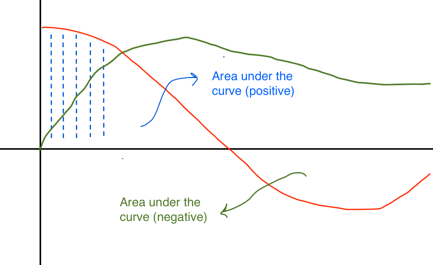 |
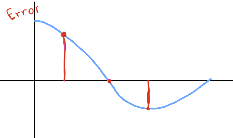
- The integral path is used to remove constant errors
- Even small errors accumulates and add up to adjust the controller output
Comments
- Not all PID paths must be present (set the corresponding constant to zero)
- Making a simple controller is better when all requirements are met
- Easy to implement
- Easy to test, tune and troubleshoot
- Easy to understand by other people
- This is also why PID are so widdespread even if there are a lot of controller types available
- The PID transfer function:
- $\tau_I, \tau_D$: integral and derivative time constant (paramenters)
- Note that the PID has one pole at the origina and two zeros in:
- This is an ideal PID;
- A real PID has high frequency poles (high frequency roll off of the frequency response)
Filtering and Set Point Weighting
- Differentiation is always sensitive to noise
Think of $G(s)=s$, whose response goes to infinity for large $s$.
In practice, when there is a derivative action we need to limit the high frequency gain.
- This can be done implementing the derivative term as:
- We are filtering the ideal derivative $K_d s$ with a first order system with time constant $\hat{K}_d/N$.
- Acts as a derivative for low-frequency signal components
- Gain is limited (depends on $\frac{K_d}{\hat{K}_d/N}$) and so is high-frequency noise
 |
- The derivative action might lead to large control outputs at high frequency
A step change in the reference signal will result in an impulse in the control signal
$$ K_d \frac{d e(t)}{dt} \rightarrow \infty $$
- A similar issue is also present in the proportional term $K_p e(t)$ which undergoes a step change in value
- In process control applications, a step change in the manipulated variable may require sudden and abrupt changes in valve position, process flows, or pressures, all of which can cause significant strain on very large devices.
- This phenomenon is called setpoint kick (or sometimes derivative kick) which is generally to be avoided.
- Setpoint Kick can be avoided filtering the reference before feeding it to the controller
- or changing the structure of the PID controller:
- $\beta$ and $\gamma$ are two additional parameters
- The effect is to introduce a different error term for each term in the control equation
- Note that the integral term must be based on error feedback to ensure the desired steady state
- The error terms for the proportional and derivative terms now include constants $\beta$ and $\gamma$ that are used to modify the response to setpoint changes.
- Common practice is to set $\gamma=0$
- Entirely eliminates derivative action based on change in the setpoint.
- When incorporated in PID control, this is also called derivative on output (and $e(t)=y(t)$)
- Almost always a good idea in process control because it eliminates the 'derivative kick' associated with a quick change in setpoint.
 |
- In practice, the term $\beta$ is generally tuned to meet the specific application requirements.
- If setpoint tracking is not a high priority, setting $\beta=0$ is a reasonable starting point.
time = np.arange(0, 10, 0.1)

e = []  # error
int_e = [] # integral of the error
int_e.append(0)

for t in time:
    e.append(0.3*(-t+5))
    int_e.append((int_e[-1]+e[-1]))
fig, axs = plt.subplots(1, figsize=(10,5))
plt.plot(time, e, color='b', label='error', linewidth=3)
plt.plot(time, int_e[:-1], color='r', label='int(e)', linewidth=3)
plt.plot(time, np.clip(np.array(int_e[:-1]), -10, 10), color='g', label='clip(int(e))', linewidth=3)
plt.grid()
plt.legend();
plt.xlabel('time');

Solutions
- Initializing the controller integral to a desired value, for instance to the value before the problem
- Zeroing the integral value every time the error is equal to, or crosses zero. This avoids having the controller attempt to drive the system to have the same error integral in the opposite direction as was caused by a perturbation
time = np.arange(0, 10, 0.1)

e = []
int_e = []
int_e.append(0)
for t in time:
    e.append(0.3*(-t+5))
    if abs(e[-1]) < 0.1:
        int_value = 0
    else:
        int_value = int_e[-1]+e[-1]
    int_e.append(int_value)
fig, axs = plt.subplots(1, figsize=(10,5))
plt.plot(time, e, color='b', label='error', linewidth=3)
plt.plot(time, int_e[:-1], color='r', label='int(e)', linewidth=3)
plt.plot(time, np.clip(np.array(int_e[:-1]), -10, 10), color='g', label='clip(int(e))', linewidth=3)
plt.grid()
plt.legend();
plt.xlabel('time');

- $G(s)$ BIBO stable
- $G(0)>0$
 |
Steps:
- Close the loop with the proportional part only
- Apply step input and increase the gain until output starts to oscillate
- Record $K^*$ (critical gain) and $T_p^*$ (oscillation period) of the output.
- Choose the PID parameters as:
| $R(s)$ | $K_p$ | $\tau_I$ | $\tau_d$ |
|---|---|---|---|
| $P$ | $0.5K^*$ | ||
| $PI$ | $0.45K^*$ | $0.8T_p^*$ | |
| $PID$ | $0.6K^*$ | $0.5T_p^*$ | $01258T_p^*$ |
- These rules do not squeeze out the best possible performance
- $K^*$ is the gain margin with a proportional controller
- Critical frequency (for which $|L(jw)|=1$ is $\frac{2\pi}{T_p^*}$
- The rules means having a 6dB gain margin
- Integral term better steady state but slows down the system (reduces bandwidth and phase margin)
Derivative term increases the bandwidth and phase margin
Not possible to use when the plant is potentially dangerous
- Plants that are difficult to bring to oscillate using a proportional controller only (1st and 2nd order with infinite gain margin)
s = control.tf([1, 0], [1])

G_s = 6.2/(2*s**3 + 3*s**2 +s + 1)

print(G_s)
Let's see what happens when we close the loop:
$$ R(s) = 1 $$Measurement $$ H(s) = 0.042 $$
Step response with no controller:
fig, ax = plt.subplots(1, figsize=(10,5))
t_out, y_out = control.step_response(control.feedback(G_s, 0.042, sign=-1), T=100)
plt.plot(t_out, y_out, linewidth=3)
plt.grid()
plt.xlabel('time');

fig, ax = plt.subplots(1, figsize=(10,5))

K_p_range = [0.1, 0.5, 1, 1.5, 1.92]
for K_p in K_p_range:
    t_out, y_out = control.step_response(control.feedback(K_p*G_s, 0.042, sign=-1), T=100)
    plt.plot(t_out, y_out, linewidth=3, label='K={}'.format(K_p))
    plt.grid()
    plt.xlabel('time');
plt.legend();

plt.plot(5.0, 15, marker='.', markersize=15, color='r')
plt.plot(13.95, 15, marker='.', markersize=15, color='r')

- Critical gain $K^*=1.92$
- Period $T_p^*=8.95$
K_star = 1.92
T_p_start = 8.95
And we can then calculate the parameter of the PID from the ZN table
K_p = 0.6*K_star
tau_I = 0.5*T_p_start
tau_d = 0.125*T_p_start

print('K_p:', K_p)
print('tau_I:', tau_I)
print('tau_d:', tau_d)
PID = K_p*(tau_I*tau_d*s**2 + tau_I*s + 1)/(tau_I*s)

# Or in the standard form:
# K_I = K_p/tau_I
# K_d = K_p/tau_d
# PID = K_p + K_I/s + K_d*s

print(PID)
control.feedback(PID*G_s, 0.042, sign=-1)
fig, ax = plt.subplots(1, figsize=(10,5))
t_out, y_out = control.step_response(control.feedback(PID*G_s, 0.042, sign=-1), T=100)

plt.plot(t_out, y_out, linewidth=3, label='PID')
plt.grid()
plt.xlabel('time');

- Performance can also be improved manually tuning the parameters further
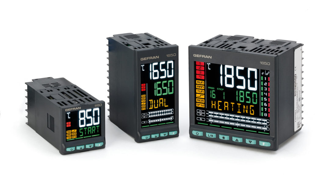
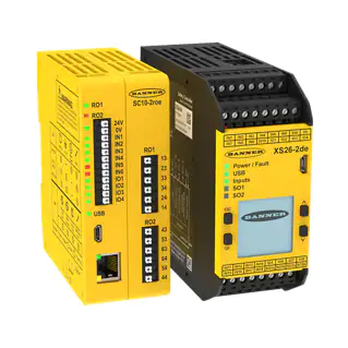
- Components are already equipped with standard controllers, of which we need to tune the parameters
- Programmable Logic Controllers (PLC) are industrial computers, ruggedized and adapted for the control of manufacturing processes
- They might include control and supervision.
| 
|
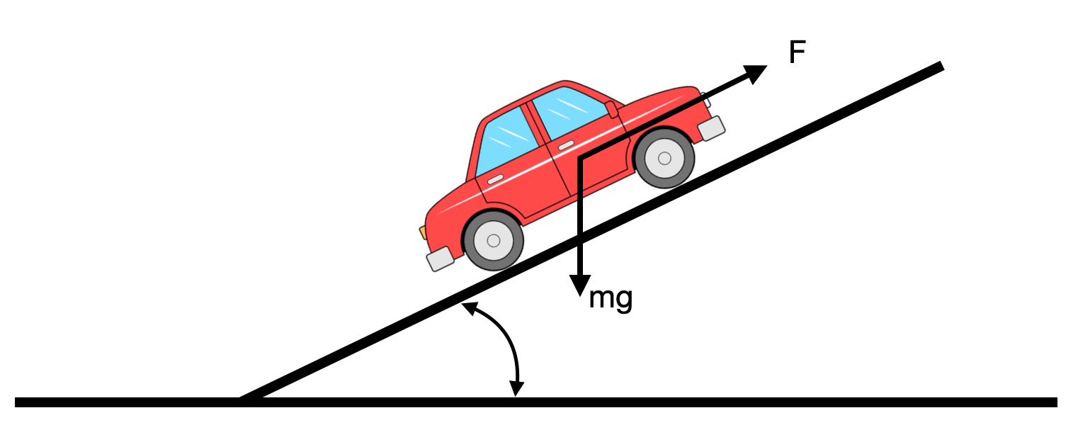 |
$$m\frac{dv}{dt} + \alpha|v|v+\beta v = \gamma u-mgsin(\theta)$$
We can linearise and calculate the transfer function from gas pedal and car velocity:
$$ G(s) = \frac{\gamma}{m}\frac{1}{s+\frac{\beta}{m}} $$And the disturbance transfer function, between slope of the road ($\theta$) and car velocity:
$$ G_d(s) = \frac{-g}{s+\frac{\beta}{m}} $$$g = 9.8m/s^2$
(see also 02_Intro_to_control_theory)
Closed loop transfer function:
| |
from classical_control_theory.intro_to_control_theory import LinearCar
m = 10
alpha = 1
beta = 1
gamma = 1
params = (m, alpha, beta, gamma)

# We select the car initial conditions (position and velocity)
x_0 = (0,0)

# We create our car
car = LinearCar(x_0, params)
theta = np.radians(20) # disturbance
u = 0                  # Input, constant and set to 0

# And finally we define the simulation parameters
t0, tf, dt = 0, 10, 0.1 # time

position = []
velocity = []
time = []
for t in np.arange(t0, tf, dt):
    car.step(dt, u, theta)
    x, y, v = car.sensor_i()
    position.append((x,y))
    velocity.append(v)
    time.append(t)

print('simulation complete')
fig, ax = plt.subplots();

plt.plot(time, velocity, linewidth=3)
plt.xlabel('time (s)')
plt.ylabel('speed (m/s)');

- Constant slope, the car rolls down
- What happens when there is no disturbance (road is flat)?
- Set
theta = np.radians(0) # disturbancein the cell above
- Set
| |
s = control.tf([1,0], [1])
G_s = 0.1/(s+0.1)

K = 5
t_out, y_out = control.step_response(control.feedback(K*G_s, 1))

print('G(s):', G_s)
print('Gcc(s):', control.feedback(K*G_s, 1))
# control.rlocus(G_s);
fig, axs = plt.subplots(1, 1, figsize=(10, 5))
plt.plot(t_out, y_out, linewidth=3)
plt.grid()
plt.title('y(end) = {}'.format(y_out[-1]));

Let's define a proportional controller in python:
def proportional(Kp, MV_bar=0):
    """Creates proportional controllers with specified gain (Kp) and setpoint (SP).
    The output is MV (manipulated variable)"""
    MV = MV_bar
    while True:
        r, y = yield MV
        MV = Kp * (r - y)
and use the car now.
We will verify how the car responds:
- with no disturbance (i.e., the slope of the road)
- without disturbance.
We will also change the controller $K$ value (e.g., 10, 20)
x_0 = (0,0)

# We create our car
car = LinearCar(x_0, params)

# We define out inputs:
theta = np.radians(0) # disturbance

# Proportional Controller
controller = proportional(Kp=5)
controller.send(None) # initialise

# Desired set point (we would like the vehicle not to move)
desired_velocity = 1

# And finally we define the simulation parameters
t0, tf, dt = 0, 10, 0.1 # time

# Simulation cycle
position = []
velocity = []
time = []
for t in np.arange(t0, tf, dt):

    u = controller.send((desired_velocity, car.speedometer()[0]))
    car.step(dt, u, theta)

    # for plotting reasons
    x, y, v = car.sensor_i()
    position.append((x,y))
    velocity.append(v)
    time.append(t)

print('simulation complete')
fig, ax = plt.subplots(1, figsize=(10, 5));

plt.plot(time, velocity, linewidth=3)
plt.xlabel('time (s)')
plt.ylabel('speed (m/s)');
plt.grid()
plt.title('velocity(end)={}'.format(velocity[-1]));

- Comments?
Let's define a PID controller in python:
def PID(Kp, Ki, Kd, MV_bar=0):
    # initialize stored data
    e_prev = 0
    t_prev = -100 # we can also set t_prev = -0.05 because in this example we are using dt=0.05
    y_prev = 0
    I = 0

    # initial control
    MV = MV_bar

    while True:
        # yield MV, wait for new t, PV, SP
        t, y, ref = yield MV

        # PID calculations
        e = ref - y

        P = Kp*e
        if t_prev >= 0:
            I = I + Ki*e*(t - t_prev)
            D = Kd*(e - e_prev)/(t - t_prev)
        else:
            I = 0
            D = 0

        MV = MV_bar + P + I + D

        # update stored data for next iteration
        e_prev = e
        t_prev = t
And simulate the PID control loop applied to the car.
We will choose arbitrary parameters $(Kp=1, Ki=1, Kd=1)$ for now, and then we will try and tune them.
x_0 = (0,0)

# We create our car
car = LinearCar(x_0, params)

# We define out inputs:
theta = np.radians(0) # disturbance
u = 0                 # Initial Input

controller = PID(1, 1, 1)        # create pid control (Kp, Ki, Kd)
controller.send(None)               # initialize

desired_velocity = 1

# And finally we define the simulation parameters
t0, tf, dt = 0, 150, 0.05 # time

position = []
velocity = []
time = []
for t in np.arange(t0, tf, dt):
    # feedback loop
    u = controller.send((t, car.speedometer()[0], desired_velocity))
    car.step(dt, u, theta)

    # plot
    x, y, v = car.sensor_i()
    position.append((x,y))
    velocity.append(v)
    time.append(t)

print('simulation complete')
fig, ax = plt.subplots(figsize=(10, 5));

plt.plot(time, velocity, linewidth=3)
plt.xlabel('time (s)')
plt.ylabel('speed (m/s)');
plt.grid();

- What happens when we add the disturbance?
- Set
theta = np.radians(20) # disturbancein the code cell to simulate the PID control loop applied to the case
- Set
Given the plant:
$$ G_{plant}(s) = \frac{K}{\tau s+1} $$Closed loop transfer function:
$$ G(s) = \frac{K\Big(K_p + \frac{K_I}{s} \big)}{\tau s+1+K\Big(K_p + \frac{K_I}{s} \big)} $$which we can write as:
$$ G(s) = \frac{K\Big(K_p s + K_I\Big)}{s^2 + (1+K K_p) s + K_I K} $$with natural frequency:
$$ w_n = \sqrt{\frac{K_IK}{\tau}} $$and
$$ \zeta = \frac{KK_p + 1}{2\sqrt{K_IK\tau}} $$The steady state error for a step input of magnitude $R$ is:
$$ e_{ss} = \lim_{s\rightarrow0} \Big[ s\Big( \frac{R}{s}-\frac{R}{s}G(s)\Big) \Big ] = 0 $$- The PI control removes the step response steady state error and allows for more control over the transient control, at least when compared with a proportional only, or integral only controller.
- For ex. it is now possible to reduce the rise time and max overshoot simultaneously.
Given:
$$ \large S = 100e^{-\frac{\zeta\pi}{\sqrt{1-\xi^2}}} $$
we can then solve for $\zeta$:
$$ \Big(\ln{\frac{S}{100}}\Big)^2 = {\zeta^2\pi^2} + \Big(\ln{\frac{S}{100}}\Big)^2 \zeta^2 $$
$$\Downarrow$$
$$ \zeta \ge \sqrt{ \frac{\Big(\ln{\frac{S}{100}}\Big)^2}{\Big(\ln{\frac{S}{100}}\Big)^2+\pi^2}} \approx 0.5 $$
Maximum desired overshoot: S=15%
S = 15 # 15%

# damping ratio:
zeta = np.sqrt(np.log(S/100)**2/(3.14**2+np.log(S/100)**2))
zeta
Given:
$$ t_r \approx \frac{1.8}{w_n} $$We can calculate the desired natural frequency for our system:
$$ w_n \approx \frac{1.8}{t_r} $$Rise time equal to $t_r=15 s$
w_n = 1.8/15
w_n
Our plant is:
$$G(s) = \frac{1}{10s+1}$$
K = 1
tau = 10
Ki = tau*w_n**2/K
Ki
Kp = (-1+2*np.sqrt(Ki*K*tau)*zeta)/K
Kp
Kd = 0 # we do not want to use the derivative path.
We can verify our performance with the Python Control Library:
PID_s = Kp + Ki/s + Kd*s

print(PID_s)
The closed loop transfer function is:
control.feedback(PID_s*G_s, 1)
And the step response:
t_out, y_out = control.step_response(control.feedback(PID_s*G_s, 1, sign=-1), T=150)
fig, ax = plt.subplots(figsize=(10, 5));

plt.plot(t_out, y_out, linewidth=3)
plt.title('max(y_out)={}'.format(max(y_out)))
plt.xlabel('time (s)')
plt.ylabel('output (m/s)');
plt.grid();

We can also plot the control command using the associated transfer function
PID_s/(1+PID_s*G_s)
t_out, y_out = control.step_response(PID_s/(1+PID_s*G_s), T=150)

fig, ax = plt.subplots(figsize=(10, 5));

plt.plot(t_out, y_out, linewidth=3)
plt.xlabel('time (s)')
plt.ylabel('control action');
plt.grid();

And finally, let's apply the calculated controller to our LinearCar
x_0 = (0,0)

# We create our car
car = LinearCar(x_0, params)

# We define out inputs:
theta = np.radians(0) # disturbance
u = 0                 # Initial Input

controller = PID(Kp=Kp, Ki=Ki, Kd=0)        # create pid control (Kp, Ki, Kd)
controller.send(None)               # initialize

desired_velocity = 1

# And finally we define the simulation parameters
t0, tf, dt = 0, 150, 0.01 # time

position = []
velocity = []
time = []
control_action = []
for t in np.arange(t0, tf, dt):
    # feedback loop
    u = controller.send((t, car.speedometer()[0], desired_velocity))
    car.step(dt, u, theta)

    # plot
    x, y, v = car.sensor_i()
    control_action.append(u)
    position.append((x,y))
    velocity.append(v)
    time.append(t)

print('simulation complete')
fig, axs = plt.subplots(2, 1, figsize=(10, 10));

axs[0].plot(time, velocity, linewidth=3)
axs[0].set_title('max(y)={}'.format(max(velocity)))
axs[0].set_ylim(0, 1.2)
axs[0].set_xlabel('time (s)')
axs[0].set_ylabel('speed (m/s)');
axs[0].grid();


axs[1].plot(time, control_action, linewidth=3)
axs[1].set_xlabel('time (s)')
axs[1].set_ylabel('control action');
axs[1].grid();

fig.tight_layout()

- We have calculated a PID controller based on a linear model of the car
- What happens when we apply it to the real, non-linear car?
| |
$$m\frac{dv}{dt} + \alpha|v|v+\beta v = \gamma u-mgsin(\theta)$$
from classical_control_theory.intro_to_control_theory import Car
Ki = 0.1440000
Kp = 0.2410951014356577
Kd = 0
PID_s = Kp + Ki/s + Kd*s
print(PID_s)
x_0 = (0,0,0)

# We create our car
car = Car(x_0, params) # before we had: LinearCar(x_0, params)

# We define out inputs:
theta = np.radians(0) # disturbance
u = 0                 # Initial Input

controller = PID(Kp=Kp, Ki=Ki, Kd=0)        # create pid control (Kp, Ki, Kd)
controller.send(None)               # initialize

desired_velocity = 1

# And finally we define the simulation parameters
t0, tf, dt = 0, 150, 0.01 # time

position = []
velocity = []
time = []
control_action = []
for t in np.arange(t0, tf, dt):
    # feedback loop
    u = controller.send((t, car.speedometer()[0], desired_velocity))
    car.step(dt, u, theta)

    # plot
    x, y, v = car.sensor_i()
    control_action.append(u)
    position.append((x,y))
    velocity.append(v)
    time.append(t)

print('simulation complete')
fig, axs = plt.subplots(2, 1, figsize=(10, 10));

axs[0].plot(time, velocity, linewidth=3)
axs[0].set_title('max(y)={}'.format(max(velocity)))
axs[0].set_ylim(0, 1.2)
axs[0].set_xlabel('time (s)')
axs[0].set_ylabel('speed (m/s)');
axs[0].grid();


axs[1].plot(time, control_action, linewidth=3)
axs[1].set_xlabel('time (s)')
axs[1].set_ylabel('control action');
axs[1].grid();

fig.tight_layout()

- The response is different. No overshoot, and no steady state error.
- What happens when we add noise? Try set
theta = np.radians(20) # disturbancein the simulation cell. You will probably need to setaxs[0].set_ylim(-5, 1.2)in the plot cell above. - Look at the control action needed when a disturbance is present.
fin